Localizing oscillatory sources using beamformer techniques
Introduction
In this tutorial we will continue working on the dataset described in the preprocessing tutorials. Below we will repeat code to select the trials and preprocess the data as described in the earlier tutorials (trigger-based trial selection, visual artifact rejection).
In this tutorial you will learn about applying beamformer techniques in the frequency domain. You will learn how to compute appropriate time-frequency windows, an appropriate head model and lead field matrix, and various options for contrasting the effect of interest against some control/baseline. Finally, you will be shown several options for plotting the results overlaid on a structural MRI.
It is expected that you understand the previous steps of preprocessing and filtering the sensor data. Some understanding of the options for computing the head model and forward lead field is also useful.
This tutorial will not cover the time-domain option for LCMV/SAM beamformers (but see this tutorial for an example on data from a Neuromag/Elekta/MEGIN system), nor for beamformers applied to evoked/averaged data (although see an example of how to calculate virtual sensors using LCMV for an example of this).
This tutorial contains hands-on material that we use for the MEG/EEG toolkit course and it is complemented by this lecture.
Background
In the Time-Frequency Analysis tutorial we identified strong oscillations in the beta band in a language paradigm. The goal of this section is to identify the sources responsible for producing this oscillatory activity. We will apply a beamformer technique. This is a spatially adaptive filter, allowing us to estimate the amount of activity at any given location in the brain. The inverse filter is based on minimizing the source power (or variance) at a given location, subject to ‘unit-gain constraint’. This latter part means that, if a source had power of amplitude 1 and was projected to the sensors by the lead field, the inverse filter applied to the sensors should then reconstruct power of amplitude 1 at that location. Beam forming assumes that sources in different parts of the brain are not temporally correlated.
The brain is divided into a regular three dimensional grid and the source strength for each grid point is computed. The method applied in this example is termed Dynamical Imaging of Coherent Sources (DICS) and the estimates are calculated in the frequency domain (Gross ET al. 2001). Other beamformer methods rely on source estimates calculated in the time domain, e.g., the Linearly Constrained Minimum Variance (LCMV) and Synthetic Aperture Magnetometry (SAM) methods (van Veen et al., 1997; Robinson and Cheyne, 1997). These methods produce a 3D spatial distribution of the power of the neuronal sources. This distribution is then overlaid on a structural image of the subject’s brain. Furthermore, these distributions of source power can be subjected to statistical analysis. It is always ideal to contrast the activity of interest against some control/baseline activity. Options for this will be discussed below, but it is best to keep this in mind when designing your experiment from the start, rather than struggle to find a suitable control/baseline after data collection.
Procedure
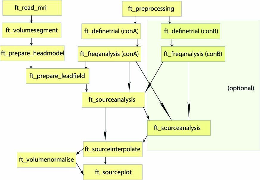
To localize the oscillatory sources for the example dataset we will perform the following steps:
- Read the data into MATLAB using ft_definetrial and ft_preprocessing
- Compute the cross-spectral density matrix using the function ft_freqanalysis
-
Construct a forward model and lead field matrix using ft_volumesegment, ft_prepare_headmodel and ft_prepare_leadfield
- Compute a spatial filter and estimate the power of the sources using ft_sourceanalysis
- Visualize the results, by first interpolating the sources to the anatomical MRI using ft_sourceinterpolate and plotting this with ft_sourceplot.
Preprocessing
The aim is to identify the sources of oscillatory activity in the beta band. From the section time-frequency analysis we have identified 18 Hz as the center frequency for which the power estimates should be calculated. We seek to compare the activation in the post-stimulus to the activation in the pre-stimulus interval. We first use ft_preprocessing and ft_selectdata to extract relevant data. It is important that the length of each data piece matches an integer number of oscillatory cycles. Here 9 cycles are used resulting in a 9/18 Hz = 0.5 s time window. Thus, the post-stimulus time-window range between 0.8 to 1.3 s and the pre-stimulus interval between -0.5 to 0.0 s (see Figure 1).
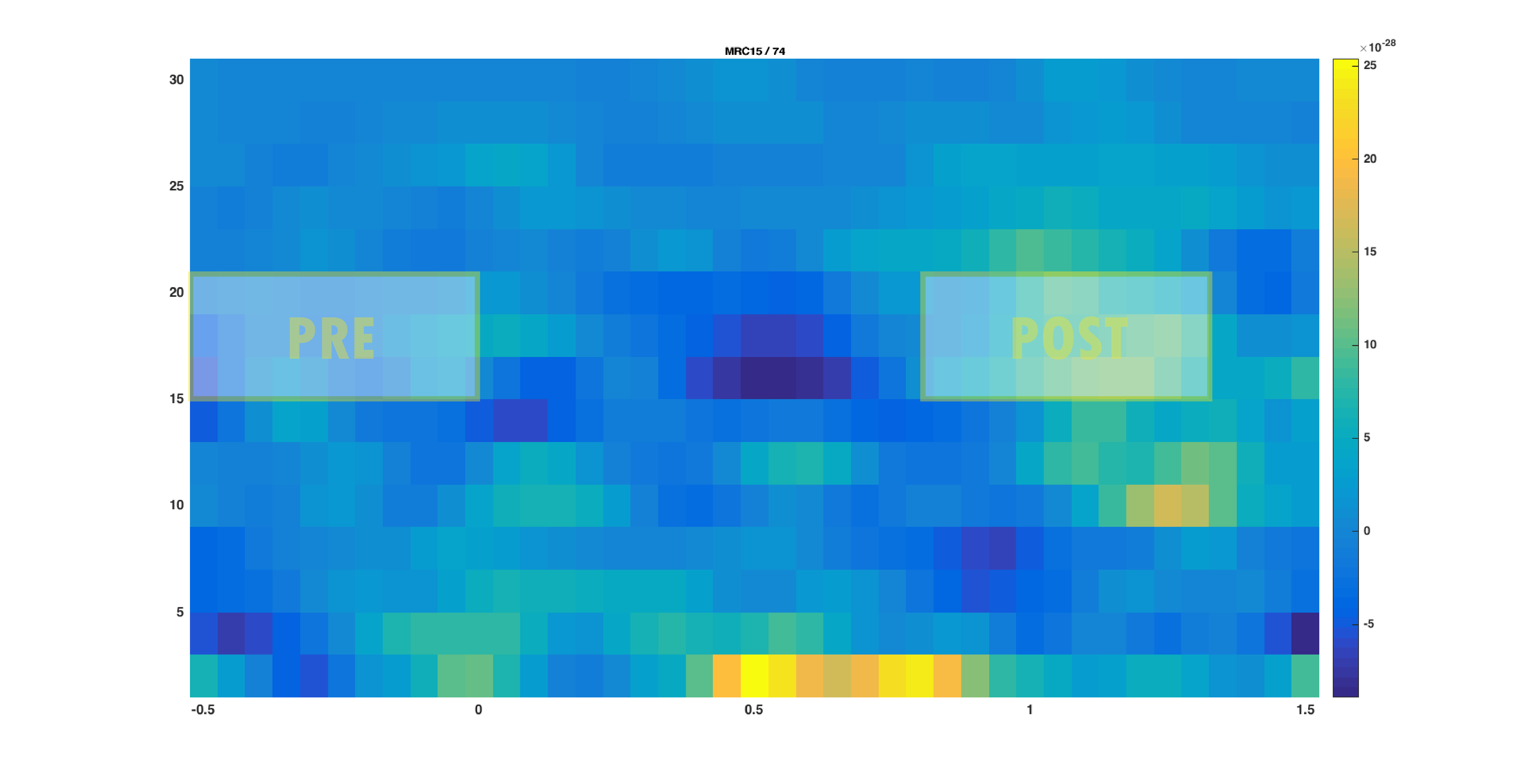
Figure 1: The time-frequency presentation used to determine the time- and frequency-windows prior to beamforming. The squares indicate the selected time-frequency tiles for the pre- and post-response..
Reading & Cleaning the data
The ft_definetrial and ft_preprocessing functions require the original MEG dataset, which is available here
Do the trial definition for the all conditions together:
cfg                         = [];
cfg.dataset                 = 'Subject01.ds';
cfg.trialfun                = 'ft_trialfun_general'; % this is the default
cfg.trialdef.eventtype      = 'backpanel trigger';
cfg.trialdef.eventvalue     = [3 5 9]; % the values of the stimulus trigger for the three conditions
% 3 = fully incongruent (FIC), 5 = initially congruent (IC), 9 = fully congruent (FC)
cfg.trialdef.prestim        = 1; % in seconds
cfg.trialdef.poststim       = 2; % in seconds

cfg = ft_definetrial(cfg);


% remove the trials that have artifacts from the trl
cfg.trl([2, 5, 6, 8, 9, 10, 12, 39, 43, 46, 49, 52, 58, 84, 102, 107, 114, 115, 116, 119, 121, 123, 126, 127, 128, 133, 137, 143, 144, 147, 149, 158, 181, 229, 230, 233, 241, 243, 245, 250, 254, 260],:) = [];


% preprocess the data
cfg.channel   = {'MEG', '-MLP31', '-MLO12'};        % read all MEG channels except MLP31 and MLO12
cfg.demean    = 'yes';                              % do baseline correction with the complete trial

data_all = ft_preprocessing(cfg);
These data have been cleaned from artifacts by removing several trials and two sensors; see the visual artifact rejection tutorial.
Select conditions and time windows of interest
We have identified the beta band effect on trials belonging to the fully incongruent condition (FIC, coded with a trigger value of 3). We will therefore now select all trials belonging to this condition based on the trigger information, which is preserved in the trialinfo field during the call to ft_preprocessing. Further we need to ‘cut’ out the time windows of interest: the pre- and post stimulus windows. We will do the selection of trials and time windows in one call to ft_selectdata:
cfg = [];
cfg.trials  = data_all.trialinfo == 3;
cfg.latency = [-0.5 0];
dataPre     = ft_selectdata(cfg, data_all);

cfg.trials  = data_all.trialinfo == 3;
cfg.latency = [0.8 1.3];
dataPost    = ft_selectdata(cfg, data_all);
Exercise 1: data length
Why is it important that the length of each data piece matches an integer number of oscillatory cycles?
The cross-spectral density matrix
The beamformer technique is based on an adaptive spatial filter. The DICS spatial filter is derived from the frequency counterpart of the covariance matrix: the cross-spectral density matrix. This matrix contains the cross-spectral densities (CSD) for all sensor combinations and is computed from the Fourier transformed data of the single trials. It is given as output when cfg.output = ‘powandcsd’. The frequency of interest is 18 Hz and the smoothing window is +/-4 Hz:
cfg = [];
cfg.method    = 'mtmfft';
cfg.output    = 'powandcsd';
cfg.tapsmofrq = 4;
cfg.foilim    = [18 18];
freqPre = ft_freqanalysis(cfg, dataPre);

cfg = [];
cfg.method    = 'mtmfft';
cfg.output    = 'powandcsd';
cfg.tapsmofrq = 4;
cfg.foilim    = [18 18];
freqPost = ft_freqanalysis(cfg, dataPost);
The output of ft_freqanalysis should be familiar to you from the tutorial for time-frequency analysis
freqPre =
struct with fields:

    label: {150x1 cell}
   dimord: 'chan_freq'
     freq: 17.8808
powspctrm: [150x1 double]
 labelcmb: {11175x2 cell}
crsspctrm: [11175x1 double]
     elec: [1x1 struct]
     grad: [1x1 struct]
      cfg: [1x1 struct]
The forward model and lead field matrix
Head model
The forward model is a prerequisite for source reconstruction. The forward model allows us to calculate an estimate of the field measured by the MEG sensors for a given current distribution. In MEG analysis a forward model is typically constructed for each subject. There are many types of forward models which to various degrees take the individual anatomy into account. Some examples of different MEG-based headmodels are given here. We will here use a semi-realistic head model developed by Nolte (2003). It is based on a correction of the lead field for a spherical volume conductor by a superposition of basis functions, gradients of harmonic functions constructed from spherical harmonics.
For more details on the following steps, you can consult the tutorial on volume conduction models for source reconstruction of MEG data.
The first step in constructing the forward model is to find the brain surface from the subjects MRI. This procedure is termed segmentation. Note that segmentation is quite time consuming and takes about 10 minutes. For the purpose of this tutorial, we have precomputed the segmentation for you. If you want to skip ahead, you can download (segmentedmri.mat)(https://download.fieldtriptoolbox.org/tutorial/beamformer/segmentedmri.mat) and directly load the segmented MRI using the command
load segmentedmri
Otherwise, segmentation involves the following steps:
First the segmentation (ft_volumesegment makes use of SPM, and in its default behavior returns a probabilistic segmentation of the grey, white and csd compartments. The necessary SPM-files are located in fieldtripXXX/external/spm8)
mri = ft_read_mri('Subject01.mri');

cfg = [];
cfg.write      = 'no';
[segmentedmri] = ft_volumesegment(cfg, mri);
Then prepare the head model from the segmented brain surface:
cfg = [];
cfg.method = 'singleshell';
headmodel = ft_prepare_headmodel(cfg, segmentedmri);
EEG headmodels
The volume conduction model created here is MEG specific and cannot be used for EEG source reconstruction. If you are interested in EEG source reconstruction methods, you can go to the corresponding EEG headmodel tutorial.
For example, if you want to do a beamformer source reconstruction on EEG data, you have to pay special attention to the EEG referencing. The forward model will be made with a common average reference (except in some rare cases like with bipolar iEEG electrode montages), i.e. the mean value over all electrodes is zero. Consequently, this also has to be true in your data.
Prior to doing the spectral decomposition with ft_freqanalysis you have to ensure with ft_preprocessing that all channels are re-referenced to the common average reference.
Furthermore, after selecting the channels you want to use in the source reconstruction (excluding the bad channels) and after re-referencing them, you should not make sub-selections of channels any more and throw out channels, because that would cause the data not be average referenced any more.
You can now visualise the headmodel together with the sensor positions:
figure
ft_plot_sens(freqPost.grad);
hold on
ft_plot_headmodel(ft_convert_units(headmodel,'cm'));
Exercise 2: head model
Why might a single sphere model be inadequate for performing beamformer estimates?
Source model and lead fields
The next step is to discretize the brain volume into a regular grid with dipoles. For each grid point the lead field matrix is calculated. It is calculated with respect to a grid with a 1 cm resolution.
Sensors MLP31 and MLO12 were removed from the data set. Thus it is essential to remove these sensors as well when calculating the lead fields.
cfg                  = [];
cfg.grad             = freqPost.grad;
cfg.headmodel        = headmodel;
cfg.reducerank       = 2;
cfg.channel          = {'MEG','-MLP31', '-MLO12'};
% use a 3-D grid with a 1 cm resolution
cfg.resolution       = 1;
cfg.sourcemodel.unit = 'cm';
sourcemodel = ft_prepare_leadfield(cfg);
If you are not contrasting the activity of interest against another condition or baseline time-window, then you may choose to normalize the lead field (cfg.normalize=’yes’), which will help control against the power bias towards the center of the head.
Source Analysis
At this point we have computed all necessary ingredients for the beamformer source analysis. As mentioned in Background, it is ideal to contrast the activity of interest against some control.
- Suitable control windows are, for example:
- Activity contrasted with baseline (example shown here dataPost - dataPre)
- Activity of condition 1 contrasted with condition 2 (example not shown)
- However, if no other suitable data condition or baseline time-window exists, then
- Activity contrasted with estimated noise (example shown below using only dataPost)
- Use normalized lead fields (see also note above and Exercise 4)
The null hypothesis for both options within (1) is that the data in both conditions are the same, and thus the best spatial filter is the one that is computed using both data conditions together (also known as ‘common filters’). This common filter is then applied separately to each condition. Hence, the parameters of your source analysis (i.e. whether to compute common filters, whether to normalize lead fields or not) might change slightly depending on which of those strategies above you decide to use. Which strategy to use, will in turn depend on your experimental design and your research question. In the following we show two possible approaches.
Source Analysis: without contrasting condition
Using the cross-spectral density and the lead field matrices a spatial filter is calculated for each grid point. By applying the filter to the Fourier transformed data we can then estimate the power for the pre- and post-stimulus activity. This results in a power estimate for each grid point. We first show the example as if you only had dataPost (and no dataPre against which to make a contrast).
cfg              = [];
cfg.method       = 'dics';
cfg.frequency    = 18;
cfg.sourcemodel  = sourcemodel;
cfg.headmodel    = headmodel;
cfg.dics.projectnoise = 'yes';
cfg.dics.lambda       = 0;

sourcePost_nocon = ft_sourceanalysis(cfg, freqPost);
The purpose of cfg.dics.projectnoise will become more clear in the section on Neural Activity Index. The purpose of lambda is discussed in Exercise 6.
Save the output:
save sourcePost_nocon sourcePost_nocon
The beamformer procedure estimates the power in the beta frequency band at each grid point in the brain volume. The grid of estimated power values can be plotted superimposed on the anatomical MRI. This requires the output of ft_sourceanalysis (see above or download sourcePost_nocon.mat) and the subject’s MRI (included in the Subject01.zip dataset).
load sourcePost_nocon
The function ft_sourceinterpolate aligns the measure of power increase with the structural MRI of the subject. The alignment is done according to the anatomical landmarks (nasion, left and right ear canal) that were both determined in the MEG measurement and in the MRI scan. Using the ft_volumereslice function before doing the interpolation ensures that the MRI is well behaved, because the reslicing causes the voxel axes to be aligned with the head coordinate axes:
mri = ft_read_mri('Subject01.mri');

cfg = [];
mri = ft_volumereslice(cfg, mri);

cfg            = [];
cfg.downsample = 2;
cfg.parameter  = 'pow';
sourcePostInt_nocon  = ft_sourceinterpolate(cfg, sourcePost_nocon, mri);
Plot the interpolated data:
cfg              = [];
cfg.method       = 'slice';
cfg.funparameter = 'pow';
ft_sourceplot(cfg, sourcePostInt_nocon);
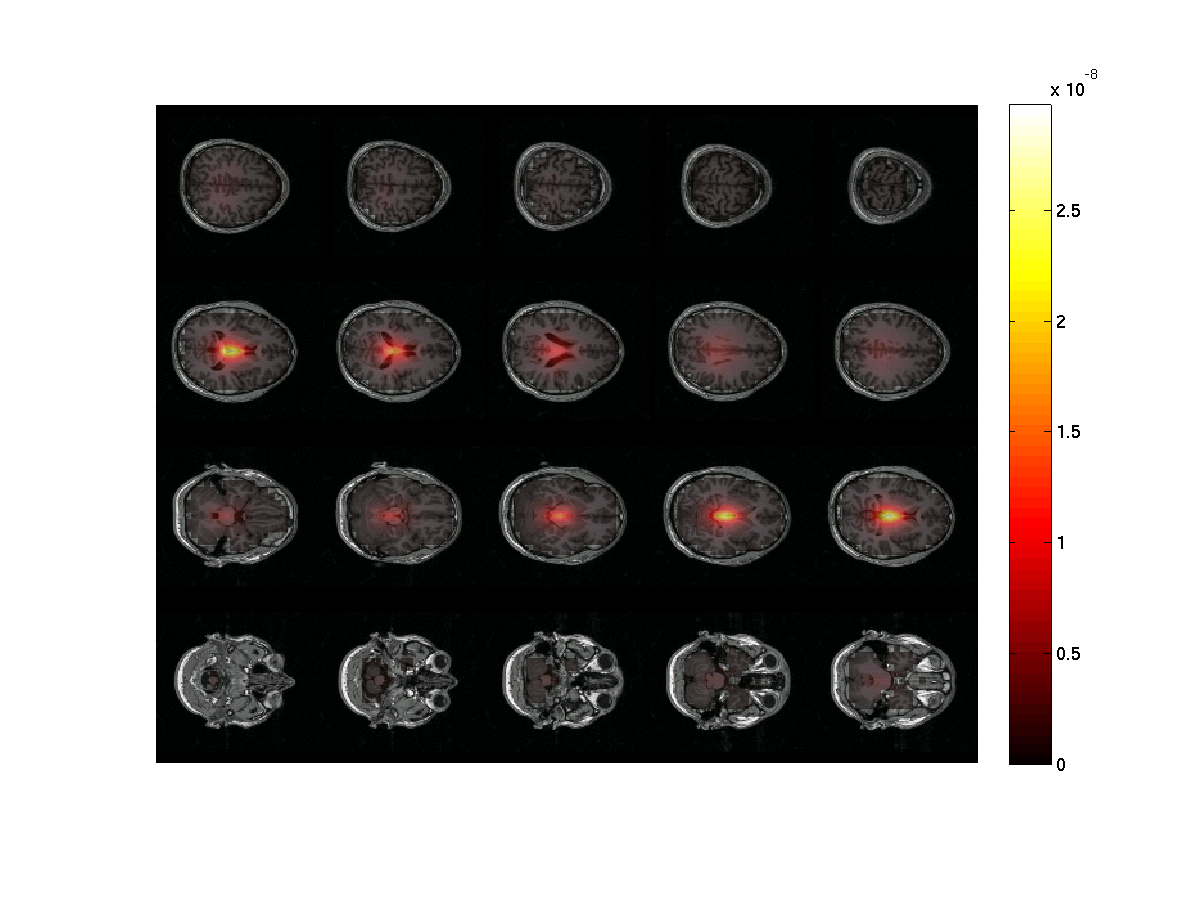
Figure 2: The power estimates of the post-stimulus activity only at ~18 Hz. Note the strong noise bias toward the center of the head. The image was done using ft_sourceinterpolate and ft_sourceplot..
Notice that the power is strongest in the center of the brain. There are several ways of circumventing the noise bias towards the center of the head which we will show below.
Exercise 3: center of head bias
Discuss why the source power is overestimated in the center of the brain. Hint 1: what are the lead field values in the center of the head? Why? Hint 2: Remember the ‘unit-gain constraint’ of beamformer spatial filters.
Neural Activity Index
If it is not possible to compare two conditions (e.g., A versus B or post versus pre) one can apply the neural activity index (NAI), in order to remove the center of the head bias shown above. The NAI is the power normalized with an estimate of the spatially inhomogeneous noise. An estimate of the noise has been done by ft_sourceanalysis, by setting cfg.dics.projectnoise=’yes’ (default is ‘no’). This noise estimate was computed on the basis of the smallest eigenvalue of the cross-spectral density matrix. To calculate the NAI do the following:
sourceNAI = sourcePost_nocon;
sourceNAI.avg.pow = sourcePost_nocon.avg.pow ./ sourcePost_nocon.avg.noise;

cfg = [];
cfg.downsample = 2;
cfg.parameter = 'pow';
sourceNAIInt = ft_sourceinterpolate(cfg, sourceNAI , mri);
Plot it:
maxval = max(sourceNAIInt.pow);

cfg = [];
cfg.method        = 'slice';
cfg.funparameter  = 'pow';
cfg.maskparameter = cfg.funparameter;
cfg.funcolorlim   = [4.0 maxval];
cfg.opacitylim    = [4.0 maxval];
cfg.opacitymap    = 'rampup';
ft_sourceplot(cfg, sourceNAIInt);
We limit the colormap for the functional data together with the opacity parameter to better see where source power is maximal. The lower limit of 4 is an arbitrary choice here. Instead, if you have a statistical map you could mask the data based on where power is significantly stronger (i.e. as compared to baseline).
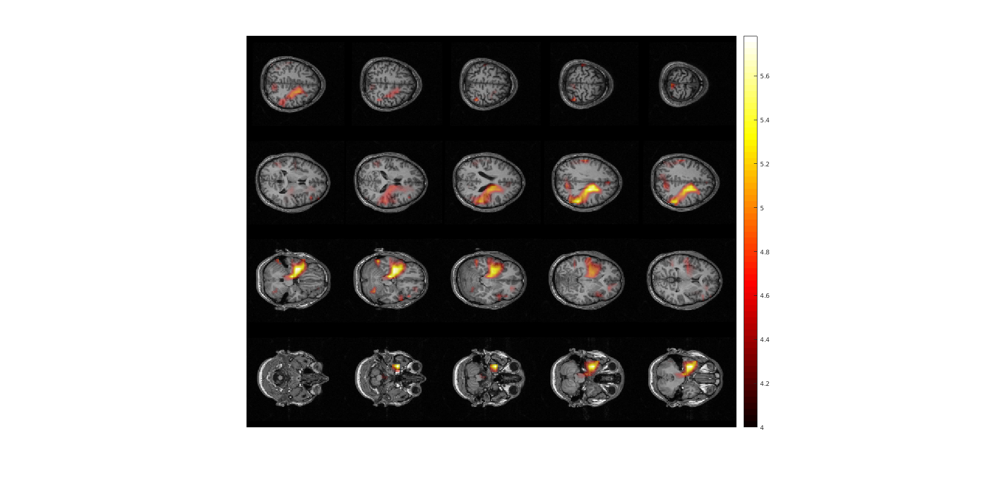
Figure 3: The neural activity index (NAI) plotted for the post-stimulus time window normalized with respect to the noise estimate.
Exercise 4: lead field normalization
Another option, besides contrasting to the noise estimate, is to normalize the lead field when you compute it (cfg.normalize=’yes’ in the call to ft_prepare_leadfield). Recompute the lead field and source estimate this way and plot the result.
Source Analysis: Contrasting activity to another interval
One approach for contrasting different intervals of the data is to compare the post- and pre-stimulus interval, which we describe now here. Another approach is to contrast the same window of interest (relative in time to some stimulus or response) between two or more conditions, which we do not show here, but the calls to FieldTrip functions are conceptually the same.
Importantly, if you later want to compare the two conditions statistically, you have to compute the sources based on an inverse filter computed from both conditions, so called ‘common filters’, and then apply this filter separately to each condition to obtain the source power estimate in each condition separately.
First we compute a single data structure with both conditions, and compute the frequency domain CSD.
dataAll = ft_appenddata([], dataPre, dataPost);

cfg = [];
cfg.method    = 'mtmfft';
cfg.output    = 'powandcsd';
cfg.tapsmofrq = 4;
cfg.foilim    = [18 18];
freqAll = ft_freqanalysis(cfg, dataAll);
Then we compute the inverse filter based on both conditions. Note the use of cfg.keepfilter so that the output saves this computed filter.
cfg              = [];
cfg.method       = 'dics';
cfg.frequency    = 18;
cfg.sourcemodel  = sourcemodel;
cfg.headmodel    = headmodel;
cfg.dics.projectnoise = 'yes';
cfg.dics.lambda       = '5%';
cfg.dics.keepfilter   = 'yes';
cfg.dics.realfilter   = 'yes';
sourceAll = ft_sourceanalysis(cfg, freqAll);
By placing this pre-computed filter inside cfg.sourcemodel.filter, it can now be applied to each condition separately.
cfg.sourcemodel.filter = sourceAll.avg.filter;
sourcePre_con  = ft_sourceanalysis(cfg, freqPre );
sourcePost_con = ft_sourceanalysis(cfg, freqPost);

save sourcePre_con sourcePre_con
save sourcePost_con sourcePost_con
Now we can compute the contrast of (post-pre)/pre. In this operation we assume that the noise bias is the same for the pre- and post-stimulus interval and it will thus be removed.
sourceDiff = sourcePost_con;
sourceDiff.avg.pow = (sourcePost_con.avg.pow - sourcePre_con.avg.pow) ./ sourcePre_con.avg.pow;
Load and reslice the MRI if not done already in previous step:
mri = ft_read_mri('Subject01.mri');
mri = ft_volumereslice([], mri);
Then interpolate the source to the MRI:
cfg            = [];
cfg.downsample = 2;
cfg.parameter  = 'pow';
sourceDiffInt  = ft_sourceinterpolate(cfg, sourceDiff , mri);
Now plot the power ratios:
maxval = max(sourceDiffInt.pow);

cfg = [];
cfg.method        = 'slice';
cfg.funparameter  = 'pow';
cfg.maskparameter = cfg.funparameter;
cfg.funcolorlim   = [0.0 maxval];
cfg.opacitylim    = [0.0 maxval];
cfg.opacitymap    = 'rampup';
ft_sourceplot(cfg, sourceDiffInt);
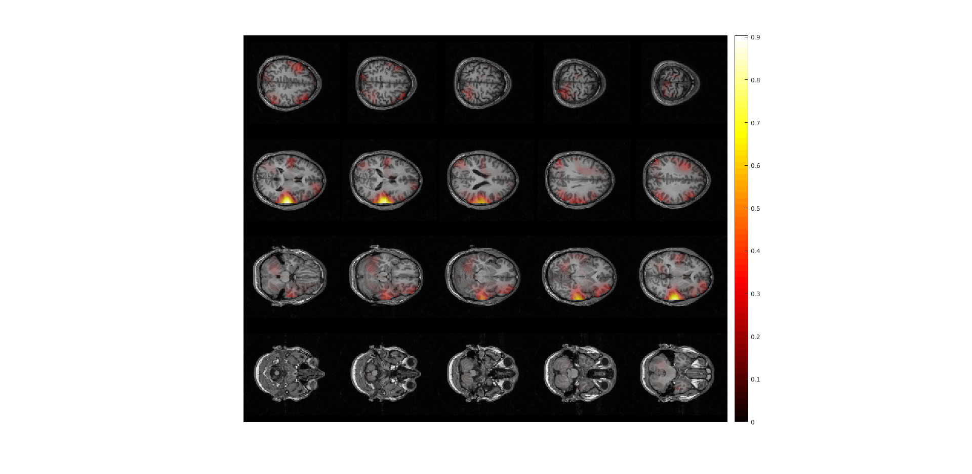
Figure 4: sourceplot with method “slice” .
Exercise 5: comparing normalizations
Compare figure 3 and 4. It appears that normalizing the power with the baseline activity result in fewer and more focal sources. Why?
Exercise 6: regularization
The regularization parameter was cfg.dics.lambda = ‘5%’. Change it to 0 or to ‘100%’ and plot the power estimate with respect to baseline. How does the regularization parameter affect the properties of the spatial filter?
Exercise 7: lead field normalization
Which configuration options you have used above for ft_sourceanalysis were specific to the type of contrast chosen?
Plotting options
To plot an ‘orthogonal’ cut
cfg = [];
cfg.method        = 'ortho';
cfg.funparameter  = 'pow';
cfg.maskparameter = cfg.funparameter;
cfg.funcolorlim   = [0.0 maxval];
cfg.opacitylim    = [0.0 maxval];
cfg.opacitymap    = 'rampup';
ft_sourceplot(cfg, sourceDiffInt);
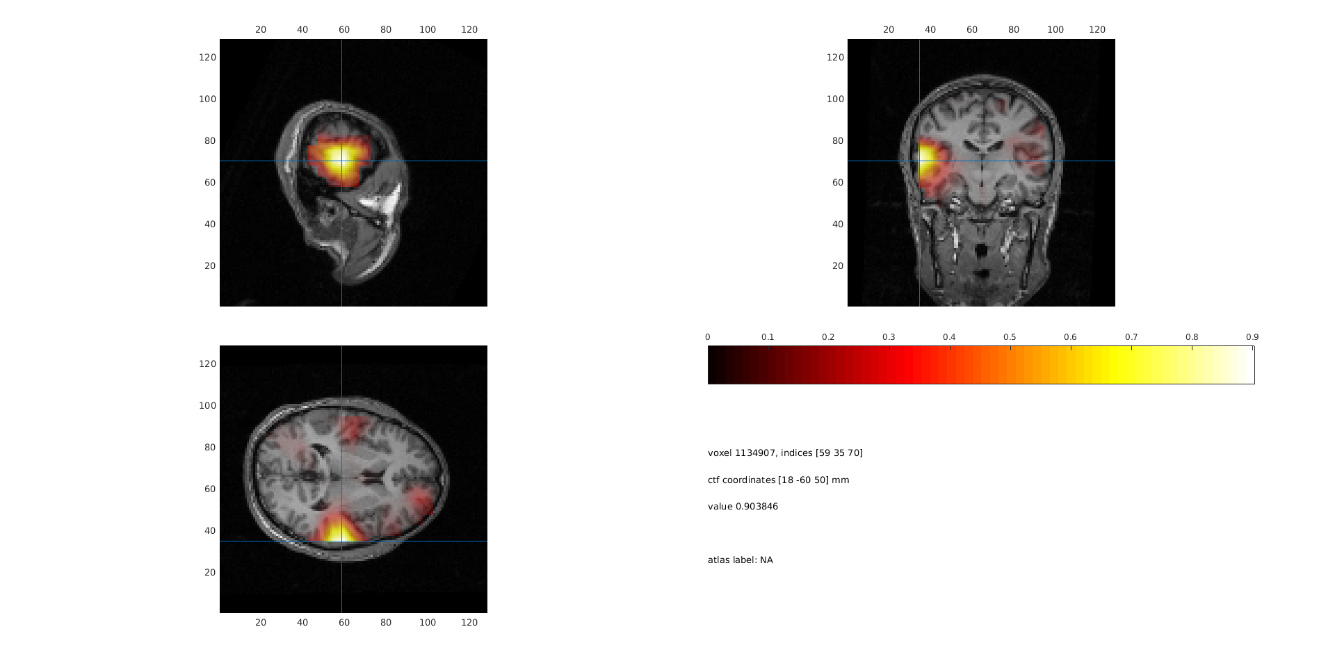
Figure 5: sourceplot with method “ortho”.
The FieldTrip function ft_volumenormalise normalises anatomical and functional volume data to a template anatomical MRI. Spatially aligning the source structures for multiple subjects allows you to compute grandaverages and over subjects statistics. Here we will illustrate the use of volume normalisation for one subject.
cfg = [];
cfg.nonlinear     = 'no';
sourceDiffIntNorm = ft_volumenormalise(cfg, sourceDiffInt);
When plotting the orthogonal view it is possible to enter interactive mode by specifying cfg.interactive=’yes’. This allows you to ‘browse’ through the brain volume by specifying the location of cut with a mouse click. To exit the interactive mode press ‘q’.
cfg = [];
cfg.method        = 'ortho';
cfg.interactive   = 'yes';
cfg.funparameter  = 'pow';
cfg.maskparameter = cfg.funparameter;
cfg.funcolorlim   = [0.0 maxval];
cfg.opacitylim    = [0.0 maxval];
cfg.opacitymap    = 'rampup';
ft_sourceplot(cfg, sourceDiffIntNorm);
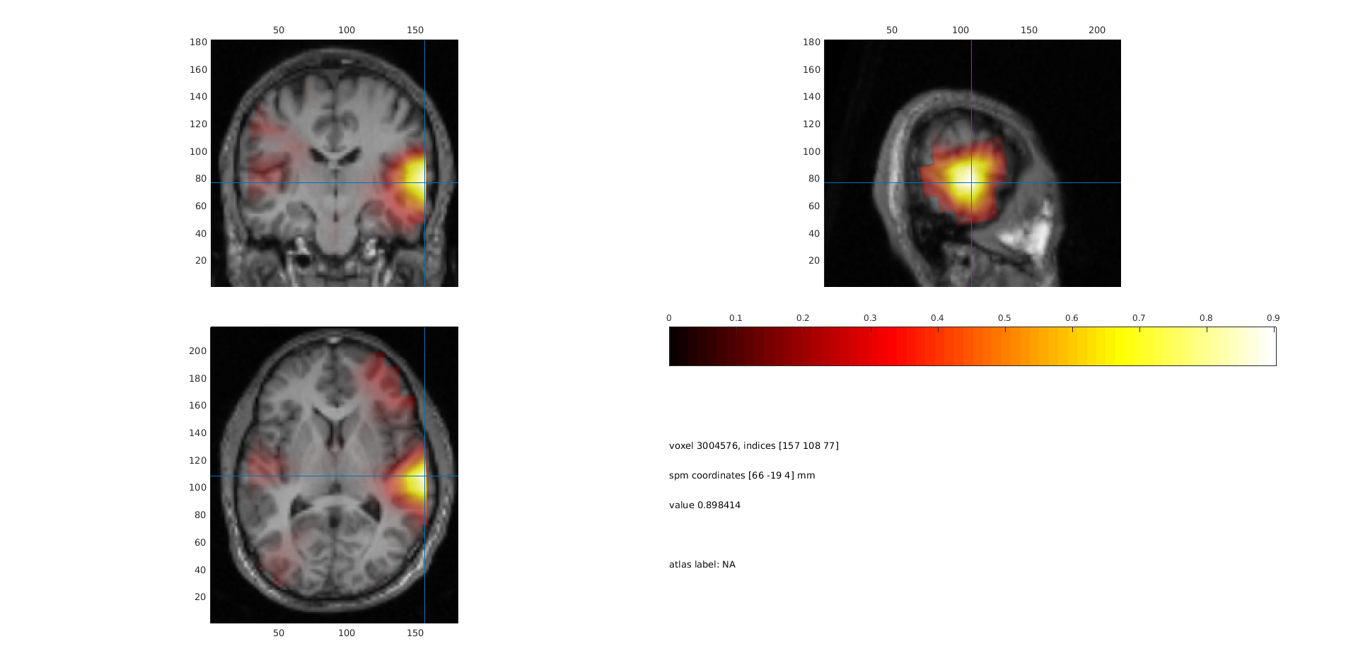
Figure 6: sourceplot with method “ortho” after volume normalisation.
You can also project the power onto a surface using ft_sourceplot. FieldTrip has several surface .mat files available. The surface files are in MNI coordinates, so therefore we use the normalized volume to match those coordinates.
Now the data can be plotted
cfg = [];
cfg.method         = 'surface';
cfg.funparameter   = 'pow';
cfg.maskparameter  = cfg.funparameter;
cfg.funcolorlim    = [0.0 maxval];
cfg.funcolormap    = 'parula';
cfg.opacitylim     = [0.0 maxval];
cfg.opacitymap     = 'rampup';
cfg.projmethod     = 'nearest';
cfg.surffile       = 'surface_white_both.mat';
cfg.surfdownsample = 10;
ft_sourceplot(cfg, sourceDiffIntNorm);
view ([90 0])
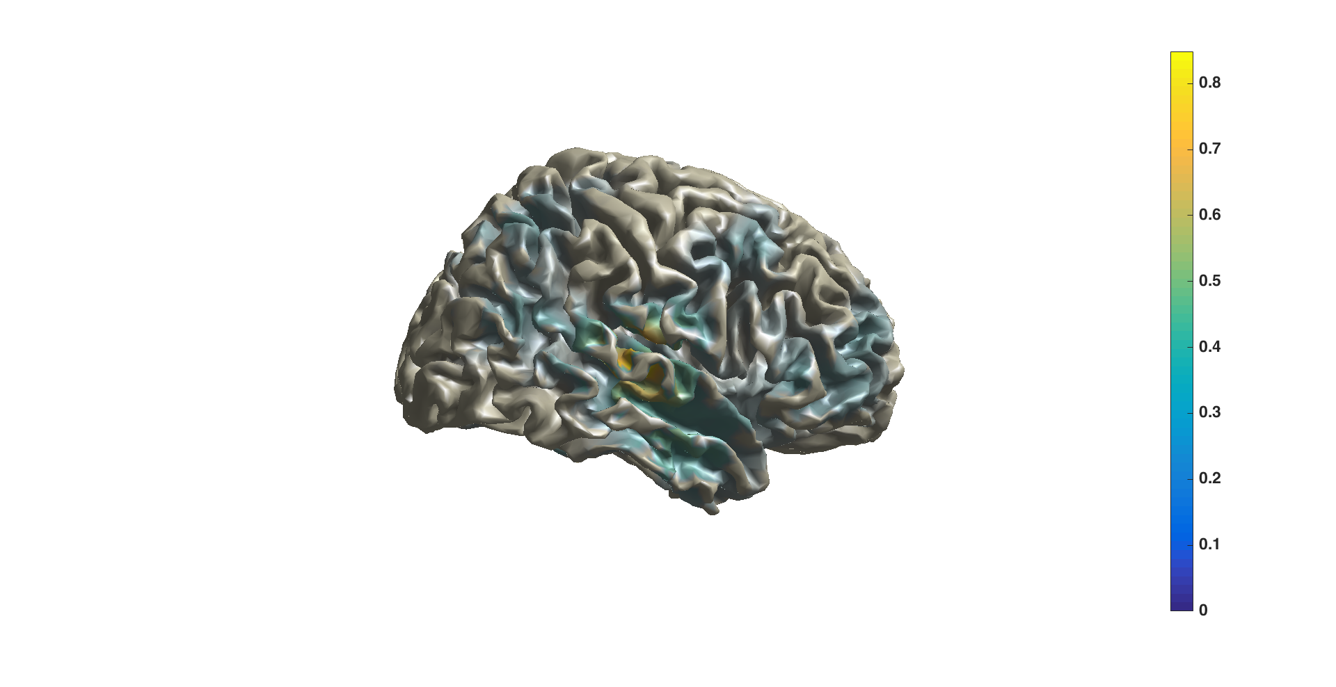
Figure 7: sourceplot with method “surface”.
Summary and suggested further reading
Beamforming source analysis in the frequency domain with DICS has been demonstrated. An example of how to compute a head model (single shell) and forward lead field was shown. Various options for contrasting the time-frequency window of interest against a control was shown, including against ‘noise’ (NAI: minimum eigenvalue of the CSD) and against the pre-stimulus window using a ‘common filter’. Options at each stage and their influence on the results were discussed, such as lead field normalization and CSD matrix regularization. Finally, options for plotting on slices, orthogonal views, or on the surface were shown.
Details on head models can be found here or here. Computing event-related fields with MNE or LCMV might be of interest. More information on common filters can be found here. If you are doing a group study where you want the grid points to be the same over all subjects, see here. See here for source statistics.
FAQs:
- Where is the anterior commissure?
- Can I do combined EEG and MEG source reconstruction?
- Can I restrict the source reconstruction to the grey matter?
- How are the different head and MRI coordinate systems defined?
- How are the Left and Right Pre-Auricular (LPA and RPA) points defined?
- How can I check whether the grid that I have is aligned to the segmented volume and to the sensor gradiometer?
- How can I determine the anatomical label of a source or electrode?
- How can I fine-tune my BEM volume conduction model?
- How can I visualize the different geometrical objects that are needed for forward and inverse computations?
- How to coregister an anatomical MRI with the gradiometer or electrode positions?
- Is it good or bad to have dipole locations outside of the brain for which the source reconstruction is computed?
- Is it important to have accurate measurements of electrode locations for EEG source reconstruction?
- What is the conductivity of the brain, CSF, skull and skin tissue?
- What kind of volume conduction models of the head (head models) are implemented?
- Where can I find the dipoli command-line executable?
- Why is there a rim around the brain for which the source reconstruction is not computed?
- Why should I use an average reference for EEG source reconstruction?
Example scripts:
- Combined EEG and MEG source reconstruction
- Common filters in beamforming
- Compute forward simulated data using ft_dipolesimulation
- Compute forward simulated data and apply a beamformer scan
- Compute forward simulated data and apply a dipole fit
- Compute forward simulated data with the low-level ft_compute_leadfield
- Check the quality of the anatomical coregistration
- Localizing the sources underlying the difference in event-related fields
- Fit a dipole to the tactile ERF after mechanical stimulation
- Align EEG electrode positions to BEM headmodel
- How to create a head model if you do not have an individual MRI
- How to import data from MNE-Python and FreeSurfer
- Make leadfields using different headmodels
- Plotting the result of source reconstruction on a cortical mesh
- Source statistics
- Create MNI-aligned grids in individual head-space
- Testing BEM created EEG lead fields
- Use your own forward leadfield model in an inverse beamformer computation