Make leadfields using different headmodels

These scripts demonstrate how to compute and compare the different MEG headmodels that are available in FieldTrip.

For all functions used, you can type 'help function' in matlab for more information.

The MEG dataset that is used in this demo is available from ftp://ftp.fcdonders.nl/pub/fieldtrip/tutorial/ and is named Subject01.zip.

If you download this data into a folder named 'testdata' the directory should look like this:

>> cd testdata
>> ls
Subject01.ds   Subject01.mri    Subject01.shape_info
Subject01.hdm  Subject01.shape

%--------------------------------------------------------------------------------------
%making a leadfield using the singleSphere headmodel that is 
%produced with CTF software
%--------------------------------------------------------------------------------------
 
%read in the single sphere models produced with ctf software
ctf_ss=ft_read_vol('Subject01.hdm');
 
%plotting the headmodel
figure;
hdr = ft_read_header('Subject01.ds');
cfg                         = [];
cfg.grad                    = hdr.grad;
cfg.headshape               = 'Subject01.shape';
cfg.vol                     = ctf_ss;
ft_headmodelplot(cfg);
title('ctf: singlesphere');
 
%prepare the leadfield for the single sphere model.
hdr = ft_read_header('Subject01.ds');
cfg                         = [];
cfg.grad                    = hdr.grad;
cfg.vol                     = ctf_ss;
cfg.resolution              = 1;
[grid_ctf_ss]=ft_prepare_leadfield(cfg);

CTF headmodel, single sphere:

%--------------------------------------------------------------------------------------
%making a leadfield using the localSpheres headmodel that is 
%produced with CTF software
%--------------------------------------------------------------------------------------
 
%read in the local spheres model produced with ctf software
ctf_ls=read_ctf_hdm('Subject01.ds/default.hdm');
 
%plotting the headmodel
figure;
hdr = ft_read_header('Subject01.ds');
cfg                       = [];
cfg.grad                  = hdr.grad;
cfg.headshape             = 'Subject01.shape';
cfg.vol                   = ctf_ls;
ft_headmodelplot(cfg);
title('ctf: localSpheres');
 
%prepare_leadfield; 
hdr = ft_read_header('Subject01.ds');
cfg                       = [];
cfg.grad                  = hdr.grad;
cfg.vol                   = ctf_ls;
cfg.resolution            = 1;
[grid_ctf_ls]=ft_prepare_leadfield(cfg);

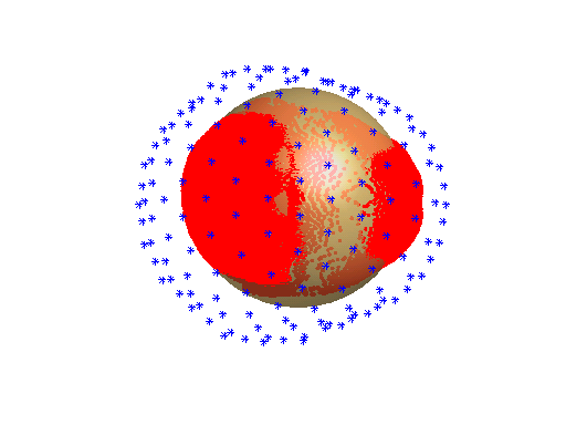
CTF headmodel, local spheres:

%--------------------------------------------------------------------------------------
%making a leadfield using ft_prepare_localspheres implemented in FieldTrip 
%using the headshape produced with CTF software
%--------------------------------------------------------------------------------------
 
%ft_prepare_localspheres (for information type 'help ft_prepare_localspheres' in matlab)
hdr = ft_read_header('Subject01.ds');
cfg                        = [];
cfg.grad                   = hdr.grad;
cfg.headshape              = 'Subject01.shape';
ft_headshape               = ft_prepare_localspheres(cfg);
 
%plotting the headmodel
figure;
hdr = ft_read_header('Subject01.ds');
cfg                        = [];
cfg.grad                   = hdr.grad;
cfg.headshape              = 'Subject01.shape';
% Michael Wibral (wibral@bic.uni-frankfurt.de)
% 2007-09-25
% the next line should read (?):
% cfg. vol = headshape; because 'ctf_ls' was defined earlier
% on and refered to the localspheres headmodel from ctf
cfg.vol                    = ctf_ls;
ft_headmodelplot(cfg);
title('fieldtrip: local spheres, ctf headshape');
 
% prepare_leadfield for local spheres headmodel with ctf headshape
hdr = ft_read_header('Subject01.ds');
cfg                        = [];
cfg.grad                   = hdr.grad;
cfg.vol                    = headshape;
cfg.resolution             = 1;
[grid_ft_headshape]        = ft_prepare_leadfield(cfg);

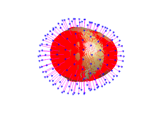
Fieldtrip headmodel, local spheres with ctf headshape:

%--------------------------------------------------------------------------------------
%making a leadfield using prepare_localspheres implemented in fieldtrip 
%using a segmented mri produced with volume_segment in fieldtrip
%(see the bottom of this page for how to make a segmented mri and check it for flipped
%dimensions)
%--------------------------------------------------------------------------------------
 
%ft_prepare_localspheres (for information type 'help ft_prepare_localspheres' in matlab)
hdr = ft_read_header('Subject01.ds');
cfg                       = [];
cfg.grad                  = hdr.grad;
ft_segment                = ft_prepare_localspheres(cfg,segmentedmri);
 
%plotting the headmodel
figure;
hdr = ft_read_header('Subject01.ds');
cfg                       = [];
cfg.grad                  = hdr.grad;
cfg.headshape             = 'Subject01.shape';
cfg.vol                   = segment;
ft_headmodelplot(cfg);
title('fieldtrip: local spheres based on segmented mri');
 
%ft_prepare_leadfield for the local spheres headmodel produced using a segmented mri
hdr = ft_read_header('Subject01.ds');
cfg                       = [];
cfg.grad                  = hdr.grad;
cfg.vol                   = segment;
cfg.resolution            = 1;
[grid_ft_segment]=ft_prepare_leadfield(cfg);

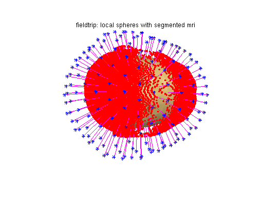
FieldTrip headmodel, local spheres based on segmented mri:

%--------------------------------------------------------------------------------------
%making a leadfield using ft_prepare_singleshell (developed by Nolte) implemented in FieldTrip 
%using a segmented mri produced with ft_volumesegment in FieldTrip
%(see the bottom of this page for how to make a segmented mri and check it for flipped
%dimensions)
%--------------------------------------------------------------------------------------
 
%ft_prepare_singleshell (for information type 'help ft_prepare_singleshell' in matlab)
hdr = ft_read_header('Subject01.ds');
cfg                       = [];
cfg.grad                  = hdr.grad;
ft_singleshell=ft_prepare_singleshell(cfg,segmentedmri);
 
%plotting the headmodel
figure;
hdr = ft_read_header('Subject01.ds');
cfg                       = [];
cfg.grad                  = hdr.grad;
cfg.headshape             = 'Subject01.shape';
cfg.vol                   = ft_singleshell;
ft_headmodelplot(cfg);
title('fieldtrip: headmodel by Nolte with segmented mri');
cfg=rmfield(cfg,'headshape');
figure;
ft_headmodelplot(cfg);
title('fieldtrip: headmodel by Nolte with segmented mri');
 
%ft_prepare_leadfield for the Nolte headmodel, created using FieldTrip
hdr = ft_read_header('Subject01.ds');
cfg                       = [];
cfg.grad                  = hdr.grad;
cfg.vol                   = ft_singleshell;
cfg.resolution            = 1;
[grid_singleshell]=ft_prepare_leadfield(cfg);

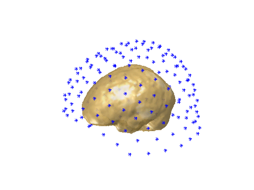
Single-shell headmodel, realistic geometry:

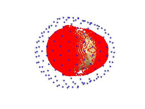
Single-shell headmodel, displayed without headshape and rotated:

%----------------------------------------------------------------------------------------------------------
%compute the amplitudes of the leadfields 
%----------------------------------------------------------------------------------------------------------
grid = {};
grid{1} = grid_ctf_ss;
grid{2} = grid_ctf_ls;
grid{3} = grid_ft_headshape;
grid{4} = grid_ft_segment;
grid{5} = grid_singleshell;
 
ampl = {};
for i.html">i=1:5
  a = grid{i.html">i};
  ampl{i.html">i} = [];
  ampl{i.html">i}.norm = zeros(grid{5}.dim) * nan;
  for k=a.inside(:)'
    ampl{i.html">i}.norm(k) = sqrt(sum(a.leadfield{k}(:).^2));
  end
end
 
%interpolating the data to the mri for plotting
mri=ft_read_mri('Subject01.mri');
cfg                        = [];
source                     = grid{1};
source.dim                 = grid{5}.dim;
sourceinterp               = {};
for i.html">i=1:5
    source.avg.pow=ampl{i.html">i}.norm;
    sourceinterp{i.html">i}=ft_sourceinterpolate(cfg,source,mri);
end
 
%plotting the correlations
cfg                        = [];
cfg.funparameter           = 'avg.pow';
cfg.nslices                = 12;
cfg.colmax                 = 1;
cfg.colmin                 = 0.8;
cfg.spacemin               = 75;
cfg.spacemax               = 150;
figure;
ft_sliceinterp(cfg,sourceinterp{1});
figure;
ft_sliceinterp(cfg,sourceinterp{2});% etcetera...

%--------------------------------------------------------------------------------------------
%compute the correlations between the different leadfields
%NOTE:to be able to compare them you should recalculate the leadfields with the grid
%specifications for the single-shell model to make the leadfields of comparable sizes: 
%in the cfg for prepare_leadfield the input should contain:
%cfg.grid.xgrid = grid_singleshell.xgrid;
%cfg.grid.ygrid = grid_singleshell.ygrid;
%cfg.grid.zgrid = grid_singleshell.zgrid;
%cfg.grid.pos = grid_singleshell.pos;
%cfg.grid.inside = grid_singleshell.inside;
%cfg.grid.outside = grid_singleshell.outside;
%cfg.resolution=[];
%--------------------------------------------------------------------------------------------
comp = {};
for i.html">i=1:5
for j.html">j=(i.html">i+1):5
  disp([i.html">i j.html">j]);
  a = grid{i.html">i};
  b = grid{j.html">j};
  comp{i.html">i,j.html">j} = [];
  comp{i.html">i,j.html">j}.corrcoef = zeros(grid{5}.dim) * nan;
  for k=a.inside(:)'
    dum = corrcoef(a.leadfield{k}(:), b.leadfield{k}(:));
    comp{i.html">i,j.html">j}.corrcoef(k) = dum(1,2);
  end
end
end
 
%interpolate the data on an mri for plotting the correlations between the leadfields
mri=ft_read_mri('Subject01.mri');
cfg                 = [];
source              = grid{1};
source.dim          = grid{5}.dim;
sourceinterp        = {};
for i.html">i=1:5
  for j.html">j=(i.html">i+1):5
    source.avg.pow=comp{i.html">i,j.html">j}.corrcoef;
    sourceinterp{i.html">i,j.html">j}=ft_sourceinterpolate(cfg,source,mri);
  end
end
 
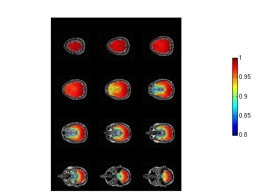
%plotting the correlations
cfg                 = [];
cfg.funparameter    = 'avg.pow';
cfg.nslices         = 12;
cfg.colmax          = 1;
cfg.colmin          = 0.8;
cfg.spacemin        = 75;
cfg.spacemax        = 150;
figure;
ft_sliceinterp(cfg,sourceinterp{1,2});
figure;
ft_sliceinterp(cfg,sourceinterp{2,3});% etcetera...

Correlations between the leadfields computed based on the FieldTrip localspheres model based on the CTF headshape and the realistic single-shell headmodel

The following code demonstrates how to make a segmented mri and check for flipped dimensions.

%-------------------------------------------------------------------------------
%make segmented mri with volumesegment
%-------------------------------------------------------------------------------
 
mri = ft_read_mri('Subject01.mri');
cfg                 = [];
cfg.name            = 'segment';
cfg.write           = 'yes';
cfg.coordinates     = 'ctf';
[segmentedmri]      = ft_volumesegment(cfg, mri)
 
%check segmented volume against mri, represent it as functional data (beamed power)
mri=ft_read_mri('Subject01.mri');
segmentedmri.avg.pow=segmentedmri.gray+segmentedmri.white+segmentedmri.csf;
segmentedmri.anatomy=mri.anatomy;
cfg              = [];
cfg.funparameter = 'avg.pow';
figure;
ft_sourceplot(cfg,segmentedmri);
 
%flip the dimensions, bug in volumesegment sometimes puts the segment upside down
test=segmentedmri;
test.gray=flipdim(segmentedmri.gray,1);
test.gray=flipdim(test.gray,2);
test.gray=flipdim(test.gray,3);
test.white=flipdim(segmentedmri.white,1);
test.white=flipdim(test.white,2);
test.white=flipdim(test.white,3);
test.csf=flipdim(segmentedmri.csf,1);
test.csf=flipdim(test.csf,2);
test.csf=flipdim(test.csf,3);
segmentedmri=test;
segmentedmri.dim=mri.dim;
segmentedmri.transform=mri.transform;
segmentedmri.anatomy=mri.anatomy;
segmentedmri.avg.pow= segmentedmri.gray+segmentedmri.white+segmentedmri.csf;
cfg=[];
figure;
cfg.funparameter = 'avg.pow';
figure;
ft_sourceplot(cfg,segmentedmri);