Analysis of sensor- and source-level connectivity
Introduction
In this tutorial we will explore different measures of connectivity, using simulated data and using source-level MEG data. You will learn how to compute various connectivity measures and how these measures can be interpreted. Furthermore, a number of interpretational problems will be addressed.
Since this tutorial focusses on connectivity measures in the frequency domain, we expect that you understand the basics of frequency domain analysis, because this is not covered by this tutorial.
Note that this tutorial does not cover all possible pitfalls associated with the analysis of connectivity and the interpretational difficulties. Although the computation of connectivity measures might be easy using FieldTrip, the interpretation of the outcomes of those measures in terms of brain networks and activity remains challenging and should be exercised with caution.
This tutorial contains hands-on material that we use for the MEG/EEG toolkit course and it is complemented by this lecture.
Background
The brain is organized in functional units, which at the smallest level consists of neurons, and at higher levels consists of larger neuronal populations. Functional localization studies consider the brain to be organized in specialized neuronal modules corresponding to specific areas in the brain. These functionally specialized brain areas (e.g., visual cortex area V1, V2, V4, MT, …) have to pass information back and forth along anatomical connections. Identifying these functional connections and determining their functional relevance is the goal of connectivity analysis and can be done using ft_connectivityanalysis and associated functions.
The nomenclature for connectivity analysis can be adopted from graph theory, in which brain areas correspond to nodes or vertices and the connections between the nodes is given by edges. One of the fundamental challenges in the analysis of brain networks from MEG and EEG data lies not only in identifying the “edges”, i.e. the functional connections, but also the “nodes”. The remainder of this tutorial will only explain the methods to characterize the edges, but will not go into details for identifying the nodes. The beamformer tutorial and corticomuscular coherence tutorial provide more pointers to localizing the nodes.
Many measures of connectivity exist, and they can be broadly divided into measures of functional connectivity (denoting statistical dependencies between measured signals, without information about causality/directionality), and measures of effective connectivity, which describe directional interactions. If you are not yet familiar with the range of connectivity measures (i.e., mutual information, coherence, granger causality), you may want to read through some of the papers listed under the method references for connectivity analysis
After the identification of the network nodes and the characterization of the edges between the nodes, it is possible to analyze and describe certain network features in more detail. This network analysis is also not covered in this tutorial, although FieldTrip provides some functionality in this direction (see ft_networkanalysis to get started).
Procedure
This tutorial consists of three parts:
-
Simulated data with directed connections: In this part we are going to simulate some data with the help of ft_connectivitysimulation and use these data to compute various connectivity metrics. As a generative model of the data we will use a multivariate autoregressive model. Subsequently, we will estimate the multivariate autoregressive model, the spectral transfer function, and the cross-spectral density matrix using the functions ft_mvaranalysis and ft_freqanalysis. In the next step we will compute and inspect various measures of connectivity with ft_connectivityanalysis and ft_connectivityplot.
-
Simulated data with common pick-up and different noise levels: In this part we are going to simulate some data consisting of an instantaneous mixture of three ‘sources’, creating a situation of common pick up. We will explore the effect of this common pick up on the consequent estimates of connectivity, and we will investigate the effect of different mixings on these estimates.
-
Connectivity between MEG virtual channel and EMG: In this part we are going to reconstruct MEG virtual channel data and estimate connectivity between this virtual channel and EMG. The data used for this part are the same as in the corticomuscular coherence tutorial.
Simulated data with directed connections
We will first simulate some data with a known connectivity structure built in. This way we know what to expect in terms of connectivity. To simulate data we use ft_connectivitysimulation. We will use an order 2 multivariate autoregressive model. The necessary ingredients are a set of NxN coefficient matrices, one matrix for each time lag. These coefficients need to be stored in the cfg.param field. Next to the coefficients we have to specify the NxN covariance matrix of the innovation noise. This matrix needs to be stored in the cfg.noisecov field.
The model we are going to use to simulate the data is as follow
x(t) = 0.8x(t-1) - 0.5x(t-2)
y(t) = 0.9y(t-1) + 0.5z(t-1) - 0.8*y(t-2)
z(t) = 0.5z(t-1) + 0.4x(t-1) - 0.2*z(t-2)
which is done using
% always start with the same random numbers to make the figures reproducible
rng default
rng(50)

cfg             = [];
cfg.ntrials     = 500;
cfg.triallength = 1;
cfg.fsample     = 200;
cfg.nsignal     = 3;
cfg.method      = 'ar';

cfg.params(:,:,1) = [ 0.8    0    0 ;
                        0  0.9  0.5 ;
                      0.4    0  0.5];

cfg.params(:,:,2) = [-0.5    0    0 ;
                        0 -0.8    0 ;
                        0    0 -0.2];

cfg.noisecov      = [ 0.3    0    0 ;
                        0    1    0 ;
                        0    0  0.2];

data              = ft_connectivitysimulation(cfg);
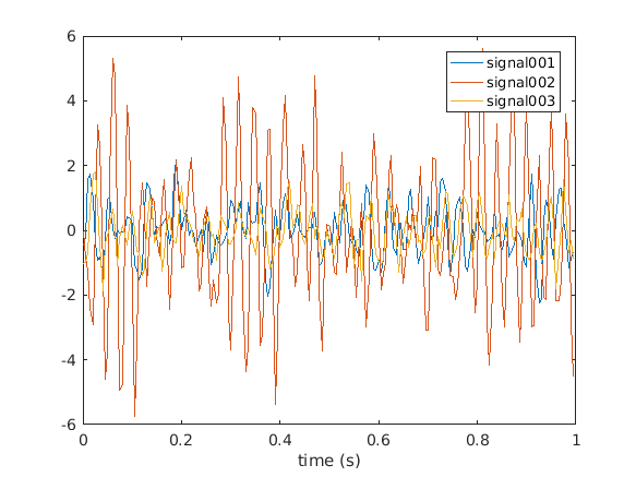
The simulated data consists of 3 channels (cfg.nsignal) in 500 trials (cfg.ntrials). You can easily visualize the data for example in the first trial using
figure
plot(data.time{1}, data.trial{1})
legend(data.label)
xlabel('time (s)')
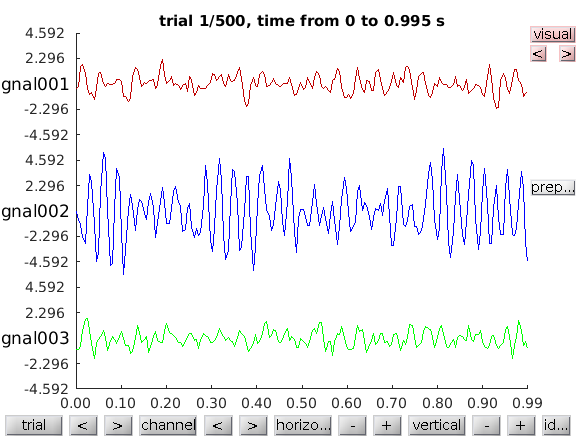
or browse through the complete data using
cfg = [];
cfg.viewmode = 'vertical';  % you can also specify 'butterfly'
ft_databrowser(cfg, data);
Computation of the multivariate autoregressive model
To be able to compute spectrally resolved Granger causality, or other frequency-domain directional measures of connectivity, we need to estimate two quantities: the spectral transfer matrix and the covariance of an autoregressive model’s residuals. We fit an autoregressive model to the data using the ft_mvaranalysis function.
For the actual computation of the autoregressive coefficients FieldTrip makes use of an implementation from third party toolboxes. At present ft_mvaranalysis supports the biosig and bsmart toolboxes for these computations.
In this tutorial we will use the bsmart toolbox. The relevant functions have been included in the FieldTrip release in the fieldtrip/external/bsmart directory. Although the exact implementations within the toolboxes differ, their outputs are comparable.
cfg         = [];
cfg.order   = 5;
cfg.toolbox = 'bsmart';
mdata       = ft_mvaranalysis(cfg, data);

mdata =
         dimord: 'chan_chan_lag'
          label: {3x1 cell}
         coeffs: [3x3x5 double]
       noisecov: [3x3 double]
            dof: 500
    fsampleorig: 200
            cfg: [1x1 struct]
The resulting variable mdata contains a description of the data in terms of a multivariate autoregressive model. For each time-lag up to the model order (cfg.order), a 3x3 matrix of coefficients is outputted. The noisecov-field contains covariance matrix of the model’s residuals.
Here, we know the model order a priori because we simulated the data and we choose a slightly higher model order (five instead of two) to get more interesting results in the output. For real data the appropriate model order for fitting the autoregressive model can vary depending on subject, experimental task, quality and complexity of the data, and model estimation technique that is used. You can estimate the optimal model order for your data by relying on information criteria methods such as the Akaike information criterion or the Bayesian information criterion. Alternatively, you can choose to use a non-parametric approach without having to decide on model order at all (see next section on Non-parametric computation of the cross-spectral density matrix)
Exercise 1
Compare the parameters specified for the simulation with the estimated coefficients and discuss.
Computation of the spectral transfer function
From the autoregressive coefficients it is now possible to compute the spectral transfer matrix, for which we use ft_freqanalysis. There are several ways of computing the spectral transfer function, the parametric and the non-parametric way. We will first illustrate the parametric route:
cfg        = [];
cfg.method = 'mvar';
mfreq      = ft_freqanalysis(cfg, mdata);

mfreq =

        freq: [1x101 double]
    transfer: [3x3x101 double]
    noisecov: [3x3 double]
   crsspctrm: [3x3x101 double]
         dof: 500
        label: {3x1 cell}
       dimord: 'chan_chan_freq'
          cfg: [1x1 struct]
The resulting mfreq data structure contains the pairwise transfer function between the 3 channels for 101 frequencies.
It is also possible to compute the spectral transfer function using non-parametric spectral factorization of the cross-spectral density matrix. For this, we need a Fourier decomposition of the data. This is done in the following section.
Non-parametric computation of the cross-spectral density matrix
Some connectivity metrics can be computed from a non-parametric spectral estimate (i.e. after the application of the FFT-algorithm and conjugate multiplication to get cross-spectral densities), such as coherence, phase-locking value and phase slope index. The following part computes the Fourier-representation of the data using ft_freqanalysis.
cfg           = [];
cfg.method    = 'mtmfft';
cfg.taper     = 'dpss';
cfg.output    = 'fourier';
cfg.tapsmofrq = 2;
freq          = ft_freqanalysis(cfg, data);

freq =
            label: {3x1 cell}
           dimord: 'rpttap_chan_freq'
             freq: [1x101 double]
    fourierspctrm: [1500x3x101 double]
        cumsumcnt: [500x1 double]
        cumtapcnt: [500x1 double]
              cfg: [1x1 struct]
The resulting freq structure contains the spectral estimate for 3 tapers in each of the 500 trials (hence 1500 estimates), for each of the 3 channels and for 101 frequencies. It is not necessary to compute the cross-spectral density at this stage, because the function used in the next step, ft_connectivityanalysis, contains functionality to compute the cross-spectral density from the Fourier coefficients.
We apply frequency smoothing of 2Hz. The tapsmofrq parameter should already be familiar to you from the multitapers section of the frequency analysis tutorial. How much smoothing is desired will depend on your research question (i.e. frequency band of interest) but also on whether you decide to use the parametric or non-parametric estimation methods for connectivity analysis:
Parametric and non-parametric estimation of Granger causality yield very comparable results, particularly in well-behaved simulated data. The main advantage in calculating Granger causality using the non-parametric technique is that it does not require the determination of the model order for the autoregressive model. When relying on the non-parametric factorization approach more data is required as well as some smoothing for the algorithm to converge to a stable result. Thus the choice of parametric vs. non-paramteric estimation of Granger causality will depend on your data and your certainty of model order. (find this information and more in Bastos and Schoffelen 2016)
Computation and inspection of the connectivity measures
The actual computation of the connectivity metric is done by ft_connectivityanalysis. This function is transparent to the type of input data, i.e. provided the input data allows the requested metric to be computed, the metric will be calculated. Here, we provide an example for the computation and visualization of the coherence coefficient.
cfg           = [];
cfg.method    = 'coh';
coh           = ft_connectivityanalysis(cfg, freq);
cohm          = ft_connectivityanalysis(cfg, mfreq);
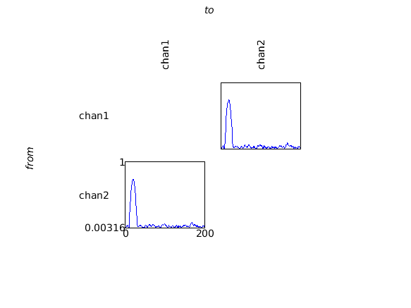
Subsequently, the data can be visualized using ft_connectivityplot.
cfg           = [];
cfg.parameter = 'cohspctrm';
cfg.zlim      = [0 1];
ft_connectivityplot(cfg, coh, cohm);
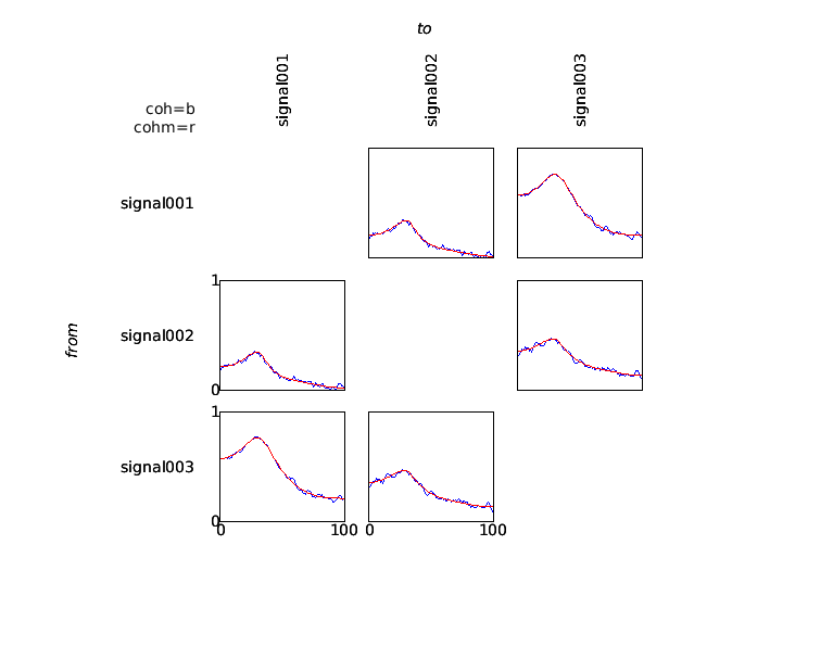
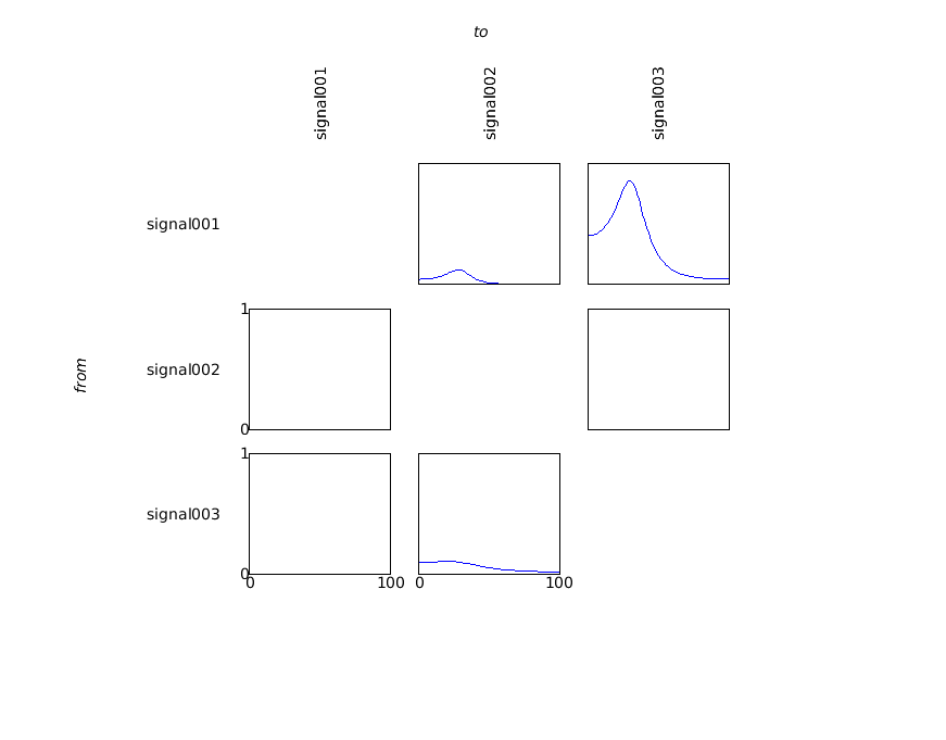
The coherence measure is a symmetric measure, which means that it does not provide information regarding the direction of information flow between any pair of signals. In order to analyze directionality in interactions, measures based on the concept of granger causality can be computed. These measures are based on an estimate of the spectral transfer matrix, which can be computed in a straightforward way from the multivariate autoregressive model fitted to the data.
cfg           = [];
cfg.method    = 'granger';
granger       = ft_connectivityanalysis(cfg, mfreq);

cfg           = [];
cfg.parameter = 'grangerspctrm';
cfg.zlim      = [0 1];
ft_connectivityplot(cfg, granger);
Exercise 2
Compute the granger output using instead the ‘freq’ data structure. Plot them side-by-side using ft_connectivityplot.
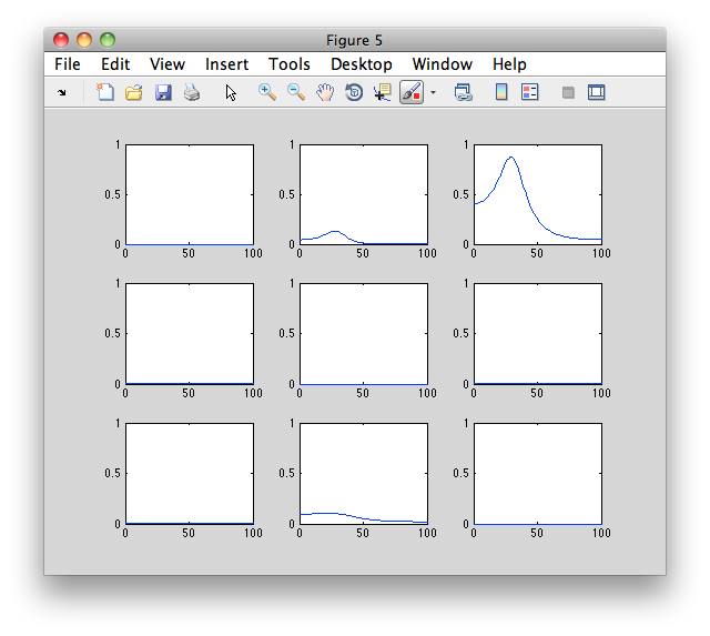
Instead of plotting it with ft_connectivityplot, you can use the following low-level MATLAB plotting code which gives a better understanding of the numerical representation of the results.
figure
for row=1:3
for col=1:3
  subplot(3,3,(row-1)*3+col);
  plot(granger.freq, squeeze(granger.grangerspctrm(row,col,:)))
  ylim([0 1])
end
end
Exercise 3
Discuss the differences between the granger causality spectra, and the coherence spectra.
Exercise 4
Compute the following connectivity measures from the mfreq data, and visualize and discuss the results: partial directed coherence (pdc), directed transfer function (dtf), phase slope index (psi). (Note that psi will require specifying cfg.bandwidth. What is the meaning of this parameter?)
Simulated data with common pick-up and different noise levels
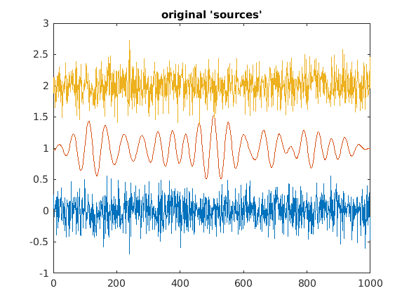
When working with electrophysiological data (EEG/MEG/LFP) the signals that are picked up by the individual channels invariably consist of instantaneous mixtures of the underlying source signals. This mixing can severely affect the outcome of connectivity analysis, and thus affects the interpretation. We will demonstrate this by simulating data in two channels, where each of the channels consists of a weighted combination of temporal white noise unique to each of the channels, and a common input of a band-limited signal (filtered between 15 and 25 Hz). We will compute connectivity between these channels, and show that the common input can give rise to spurious estimates of connectivity.
% create some instantaneously mixed data

% define some variables locally
nTrials  = 100;
nSamples = 1000;
fsample  = 1000;

% mixing matrix
mixing   = [0.8 0.2 0;
              0 0.2 0.8];

data       = [];
data.trial = cell(1,nTrials);
data.time  = cell(1,nTrials);
for k = 1:nTrials
  dat = randn(3, nSamples);
  dat(2,:) = ft_preproc_bandpassfilter(dat(2,:), 1000, [15 25]);
  dat = 0.2.*(dat-repmat(mean(dat,2),[1 nSamples]))./repmat(std(dat,[],2),[1 nSamples]);
  data.trial{k} = mixing * dat;
  data.time{k}  = (0:nSamples-1)./fsample;
end
data.label = {'chan1' 'chan2'}';

figure;plot(dat'+repmat([0 1 2],[nSamples 1]));
title('original ''sources''');

figure;plot((mixing*dat)'+repmat([0 1],[nSamples 1]));
axis([0 1000 -1 2]);
set(findobj(gcf,'color',[0 0.5 0]), 'color', [1 0 0]);
title('mixed ''sources''');

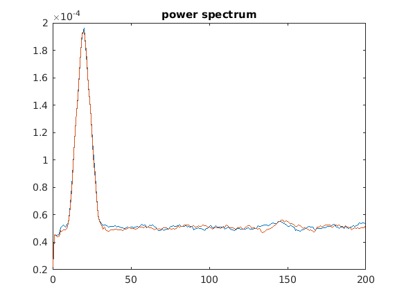
% do spectral analysis
cfg = [];
cfg.method    = 'mtmfft';
cfg.output    = 'fourier';
cfg.foilim    = [0 200];
cfg.tapsmofrq = 5;
freq          = ft_freqanalysis(cfg, data);
fd            = ft_freqdescriptives(cfg, freq);

figure;plot(fd.freq, fd.powspctrm);
set(findobj(gcf,'color',[0 0.5 0]), 'color', [1 0 0]);
title('power spectrum');
% compute connectivity
cfg = [];
cfg.method = 'granger';
g = ft_connectivityanalysis(cfg, freq);
cfg.method = 'coh';
c = ft_connectivityanalysis(cfg, freq);
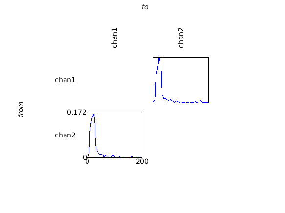
% visualize the results
cfg = [];
cfg.parameter = 'grangerspctrm';
figure; ft_connectivityplot(cfg, g);
cfg.parameter = 'cohspctrm';
figure; ft_connectivityplot(cfg, c);
Exercise 5
Simulate new data using the following mixing matrix:
[0.9 0.1 0;0 0.2 0.8]
and recompute the connectivity measures. Discuss what you see.
Exercise 6
Play a bit with the parameters in the mixing matrix and see what is the effect on the estimated connectivity.
Exercise 7
Simulate new data where the 2 mixed signals are created from 4 underlying sources, and where two of these sources are common input to both signals, and where these two sources are temporally shifted copies of one another.
Hint: the mixing matrix could look like this:
[a b c 0; 0 d e f];
and the trials could be created like this:
for k = 1:nTrials
  dat = randn(4, nSamples+10);
  dat(2,:) = ft_preproc_bandpassfilter(dat(2,:), 1000, [15 25]);
  dat(3,1:(nSamples)) = dat(2,11:(nSamples+10));
  dat = dat(:,1:1000);
  dat = 0.2.*(dat-repmat(mean(dat,2),[1 nSamples]))./repmat(std(dat,[],2),[1 nSamples]);
  data.trial{k} = mixing * dat;
  data.time{k}  = (0:nSamples-1)./fsample;
end
Compute connectivity between the signals and discuss what you observe. In particular, also compute measures of directed interaction.
Connectivity between MEG virtual channel and EMG
The previous two examples were using simulated data, either with a clear directed connectivity structure, or with a trivial pick-up of a common source in two channels. We will now continue with connectivity analysis on real MEG data. The dataset is the same as the one used in the Analysis of corticomuscular coherence tutorial.
In short, the dataset consists of combined MEG and EMG recordings while the subject lifted his right hand. The coherence tutorial contains a more elaborate description of the experiment and the dataset and a detailed analysis can be found in the corresponding paper (Jan-Mathijs Schoffelen, Robert Oostenveld and Pascal Fries. Neuronal Coherence as a Mechanism of Effective Corticospinal Interaction, Science 2005, Vol. 308 no. 5718 pp. 111-113). Due to the long distance between the EMG and the MEG, there is no volume conduction and hence no common pick-up. Hence this dataset lends itself well for connectivity analysis. But rather than using one of the MEG channels (as in the original study) and computing connectivity between that one channel and EMG, we will extract the cortical activity using a beamformer virtual channel.
Compute the spatial filter for the region of interest
We start with determining the motor cortex as the region of interest. At the end of the coherence tutorial it is demonstrated how to make a 3-D reconstruction of the cortico-muscular coherence (CMC) using the DICS algorithm. That source reconstruction serves as starting point for this analysis.
You can download the (source.mat)(https://download.fieldtriptoolbox.org/tutorial/connectivity/source.mat) file with the result from the DICS reconstruction.
We will first determine the position on which the cortico-muscular coherence is the largest.
load source

[maxval, maxindx] = max(source.avg.coh);
maxpos = source.pos(maxindx,:)

maxpos =
    4 -3 12
The cortical position is expressed in individual subject head-coordinates and in centimeter. Relative to the center of the head (in between the ears) the position is 4 cm towards the nose, -3 towards the left side (i.e., 3 cm towards the right!) and 12 cm towards the vertex.
The ft_sourceanalysis methods are usually applied to the whole brain using a regular 3-D grid or using a triangulated cortical sheet. You can also just specify the location of a single or multiple points of interest with cfg.sourcemodel.pos and the LCMV beamformer will simply be performed at the location of interest.
The LCMV beamformer spatial filter for the location of interest will pass the activity at that location with unit-gain, while optimally suppressing all other noise and other source contributions to the MEG data. The LCMV implementation in FieldTrip requires the data covariance matrix to be computed with ft_timelockanalysis.
Rather than doing all the preprocessing again, you can download the preprocessed data and headmodel data.mat and SubjectCMC.hdm.
load data

%% compute the beamformer filter
cfg                   = [];
cfg.covariance        = 'yes';
cfg.channel           = 'MEG';
cfg.covariancewindow  = 'all';
timelock              = ft_timelockanalysis(cfg, data);

cfg                  = [];
cfg.method           = 'lcmv';
cfg.hdmfile          = 'SubjectCMC.hdm';
cfg.sourcemodel.pos  = maxpos;
cfg.sourcemodel.unit = 'cm';;
cfg.keepfilter       = 'yes';
source               = ft_sourceanalysis(cfg, timelock);
The source reconstruction contains the estimated power and the source-level time series of the averaged ERF, but here we are not interested in those. The cfg.keepfilter option results in the spatial filter being kept in the output source structure. This filter can be used to reconstruct the single-trial time series as a virtual channel by multiplying it with the original MEG data.
In this case, the headmodel coordinates were defined in cm, this might be different for different headmodels. You can inspect the units of the headmodel with ft_read_headmodel
hdm = ft_read_headmodel('SubjectCMC.hdm')

hdm =
  orig: [1x1 struct]
 label: {1x183 cell}
     r: [183x1 double]
     o: [183x3 double]
  unit: 'cm'
  cond: 1
Extract the virtual channel time series
%% construct the 3-D virtual channel at the location of interest
beamformer = source.avg.filter{1};

chansel = ft_channelselection('MEG', data.label); % find the names
chansel = match_str(data.label, chansel);         % find the indices

sourcedata = [];
sourcedata.label = {'x', 'y', 'z'};
sourcedata.time = data.time;
for i=1:length(data.trial)
  sourcedata.trial{i} = beamformer * data.trial{i}(chansel,:);
end
The LCMV spatial filter is computed using data in the time domain. However, no time-domain spatial filters (during preprocessing e.g., low-pass or high-pass filters) have been applied before hand. Consequently, the filter will suppress all noise in the data in all frequency bands. The spatial filter derived from the broadband data allows us to compute a broadband source level time series.
If you would know that the subsequent analysis would be limited to a specific frequency range in the data (e.g., everything above 30 Hz), you could first apply a filter using ft_preprocessing (e.g., cfg.hpfilter=yes and cfg.hpfreq=30) prior to computing the covariance and the spatial filter.
The sourcedata structure resembles the raw-data output of ft_preprocessing and consequently can be used in any follow-up function. You can for example visualize the single-trial virtual channel time series using ft_databrowser:
cfg = [];
cfg.viewmode = 'vertical';  % you can also specify 'butterfly'
ft_databrowser(cfg, sourcedata);
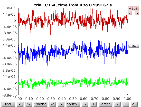
Notice that the reconstruction contains three channels, for the x-, the y- and the z-component of the equivalent current dipole source at the location of interest.
Project along the strongest dipole direction
The interpretation of connectivity is facilitated if we can compute it between two plain channels rather than between one channel and a triplet of channels. Therefore we will project the time series along the dipole direction that explains most variance. This projection is equivalent to determining the largest (temporal) eigenvector and can be computationally performed using the singular value decomposition (svd).
%% construct a single virtual channel in the maximum power orientation
timeseries = cat(2, sourcedata.trial{:});

[u, s, v] = svd(timeseries, 'econ');

whos u s v
 Name           Size              Bytes  Class     Attributes

   s              3x3                  72  double
   u              3x3                  72  double
   v         196800x3             4723200  double
Matrix u contains the spatial decomposition, matrix v the temporal and on the diagonal of matrix s you can find the eigenvalues. See help svd for more details.
We now recompute the virtual channel time series, but now only for the dipole direction that has the most power.
% this is equal to the first column of matrix V, apart from the scaling with s(1,1)
timeseriesmaxproj = u(:,1)' * timeseries;

virtualchanneldata = [];
virtualchanneldata.label = {'cortex'};
virtualchanneldata.time = data.time;
for i=1:length(data.trial)
  virtualchanneldata.trial{i} = u(:,1)' * beamformer * data.trial{i}(chansel,:);
end
Exercise 8
Rather than using a sourcemodel in the beamformer that consists of all three (x, y, z) directions, you can also have the beamformer compute the filter for only the optimal source orientation. This is implemented using the cfg.lcmv.fixedori=’yes’ option.
Recompute the spatial filter for the optimal source orientation and using that spatial filter (a 1x151 vector) recompute the time series.
Investigate and describe the difference between the two time series. What is the difference between the two dipole orientations?
Note that one orientation is represented in the SVD matrix “u” and the other is in the source.avg.ori field.
Combine the virtual channel with the EMG
The raw data structure containing one (virtual) channel can be combined with the two EMG channels from the original preprocessed data.
%% select the two EMG channels
cfg = [];
cfg.channel = 'EMG';
emgdata = ft_selectdata(cfg, data);

%% combine the virtual channel with the two EMG channels
cfg = [];
combineddata = ft_appenddata(cfg, virtualchanneldata, emgdata);

save combineddata combineddata
Compute the connectivity
The resulting combined data structure has three channels: the activity from the cortex, the left EMG and the right EMG. We can now continue with regular channel-level connectivity analysis.
%% compute the spectral decomposition
cfg            = [];
cfg.output     = 'fourier';
cfg.method     = 'mtmfft';
cfg.foilim     = [5 100];
cfg.tapsmofrq  = 5;
cfg.keeptrials = 'yes';
cfg.channel    = {'cortex' 'EMGlft' 'EMGrgt'};
freq    = ft_freqanalysis(cfg, combineddata);

cfg = [];
cfg.method = 'coh';
coherence = ft_connectivityanalysis(cfg, freq);
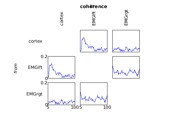
This computes the spectral decomposition and the coherence spectrum between all channel pairs, which can be plotted with
cfg = [];
cfg.zlim = [0 0.2];
figure
ft_connectivityplot(cfg, coherence);
title('coherence')
To look in more detail into the numerical representation of the coherence results, you can use
figure
plot(coherence.freq, squeeze(coherence.cohspctrm(1,2,:)))
title(sprintf('connectivity between %s and %s', coherence.label{1}, coherence.label{2}));
xlabel('freq (Hz)')
ylabel('coherence')
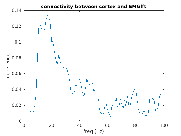
The spectrum reveals coherence peaks at 10 and 20 Hz (remember that the initial DICS localizer was done at beta). Furthermore, there is a broader plateau of coherence in the gamma range from 40-50 Hz.
Exercise 9
The spectral decomposition was performed with mutitapering and 5 Hz spectral smoothing (i.e. 5Hz in both directions). Recompute the spectral decomposition and the coherence with a hanning taper. Recompute it with mutitapering and 10 Hz smoothing. Plot the three coherence spectra and look at the differences.
Exercise 10
Rather than looking at undirected coherence, the virtual channel level data can now also easily be submitted to directed connectivity measures. Compute the spectrally resolved granger connectivity and try to assess whether the directionality is from cortex to EMG or vice versa.
Exercise 11
Let’s say you wanted to look at cortico-cortical connectivity, e.g., interactions between visual and motor cortex in a particular frequency band. How would you approach this?
Summary and further reading
This tutorial demonstrates how to compute connectivity measures between two time series. If you want to learn how to make a distributed representation of connectivity throughout the whole brain, you may want to continue with the corticomuscular coherence tutorial.
FAQs:
- How to interpret the sign of the phase slope index?
- In what way can frequency domain data be represented in FieldTrip?
- How can I compute inter-trial coherence?
- What is the difference between coherence and coherency?
Example scripts: