FieldTrip

If you use 'mtmconvol' as a method for frequency analysis it could happen that the Time-Frequency Representation of your data looks like this:

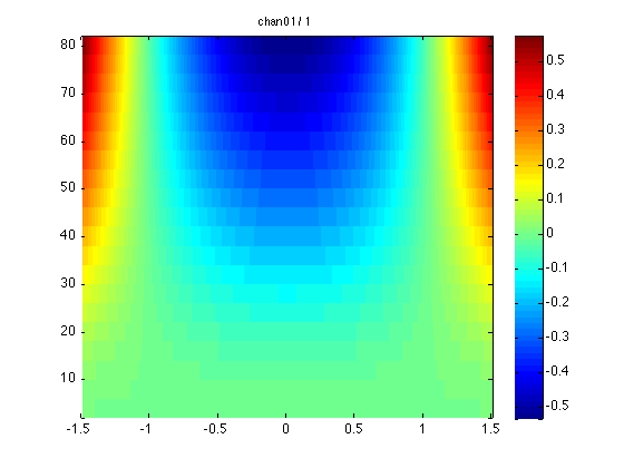
This phenomenon is caused by the time domain data having a slow low-frequency drift. This low-frequency component leaks into the estimates of all time-frequency points in a variable (but patterned) way. The reason why this actually happens is related to the fact that none of the tapered basis functions (i.e. windowed sine and cosine waves of increasing frequency) are exactly orthogonal to this slow drift. The solution to this problem is to detrend or high-pass filter your data your data prior to calling ft_freqanalysis:

cfg = [];
cfg.detrend = 'yes';
data = ft_preprocessing(cfg, data);

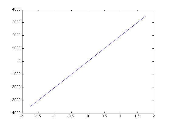
The following code shows the effect of a large amplitude low-frequency drift on the TFR:

% create some data
data = [];
data.time{1}  = [-1749:1750]./1000;
data.trial{1} = -3499:2:3499;
data.fsample  = 1000;
data.label    = {'chan01'};
figure;plot(data.time{1}, data.trial{1});

% do spectral analysis
cfg        = [];
cfg.method = 'mtmconvol';
cfg.toi    = -1.5:0.005:1.5;
cfg.foi    = 4:4:80;
cfg.t_ftimwin = ones(1,numel(cfg.foi)).*0.5;
cfg.taper  = 'hanning';
cfg.polyremoval = -1;
freq       = ft_freqanalysis(cfg, data);

% plot
cfg = [];
cfg.baseline = [-1.5 -0.5];
cfg.baselinetype = 'relchange';
figure;ft_singleplotTFR(cfg, freq);

Note that I specified the option cfg.polyremoval to be -1. This option has been introduced in July 2011, and is intended in its default behavior (the value in the default case is 1) to subtract first order linear trends from the data prior to the spectral analysis, thus aiming to avoid these surprising effects. A value of -1 is NOT the default behavior, because it will lead to no trend removal whatsoever, and therefore shows the strange behavior. The default value (which means that you don't have to worry about this) is 1, but you can also specify a higher value (removing higher order polynomes), a value of 0 (only removing the mean), or -1 (no removal at all).