Why does my TFR look strange (part I, demeaning)?
If you use ‘mtmconvol’ as a method for frequency analysis it could happen that the Time-Frequency Representation of your data looks like this:
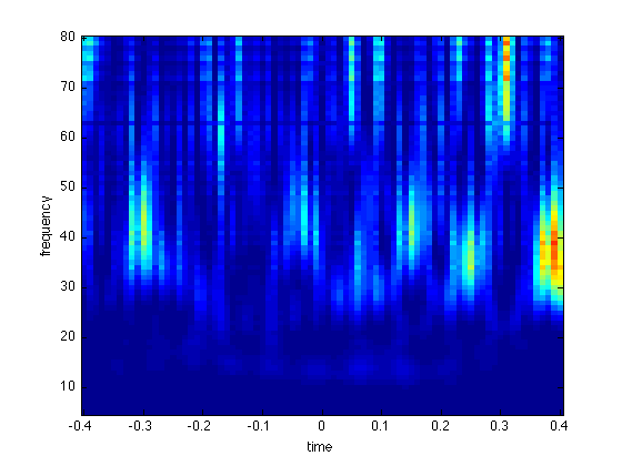
This phenomenon is caused by the time domain data having a non-zero DC component. This component leaks into the estimates of all time-frequency points in a variable (but patterned) way. The reason why this actually happens is related to the exact algorithm with which the TFR is computed in ft_freqanalysis_mtmconvol. The algorithm takes (computational) advantage of the fact that convolution in the time domain is mathematically equivalent to multiplication in the frequency domain. To this end, a fast fourier transform is applied to the time domain data, and it is combined with the fourier transform of the tapered basis functions. Importantly, no taper is applied to the data prior to fourier transformation. This leads to spectral leakage of the DC component across the whole frequency range.
The solution to this problem is to demean your data prior to calling ft_freqanalysis:
cfg = [];
cfg.demean = 'yes';
data = ft_preprocessing(cfg, data);
The following code shows the effect of a non-zero DC component on the TFR:
% create some data
data=[];
data.trial{1}     = randn(1,1000) + 2.*ft_preproc_bandpassfilter(randn(1,1000), 1000, [25 45]); %chan01 no DC component
data.trial{1}(2,:)= data.trial{1}(1,:)+100; % introduce big DC component in chan02
data.label        = {'chan01';'chan02'}
data.time{1}      = -0.5:0.001:0.499;
data.fsample      = 1000;

% do tfr-decomposition
cfg        = [];
cfg.method = 'mtmconvol';
cfg.toi    = -0.4:0.01:0.4;
cfg.foi    = 5:80;
cfg.taper  = 'hanning';
cfg.t_ftimwin = 4./cfg.foi;
cfg.polyremoval = -1; % see below
freq       = ft_freqanalysis(cfg, data)

% plot
figure;imagesc(freq.time,freq.freq,squeeze(freq.powspctrm(1,:,:)));axis xy; caxis([0 0.6]);
xlabel('time');ylabel('frequency');
figure;imagesc(freq.time,freq.freq,squeeze(freq.powspctrm(2,:,:)));axis xy; caxis([0 0.6]);
xlabel('time');ylabel('frequency');
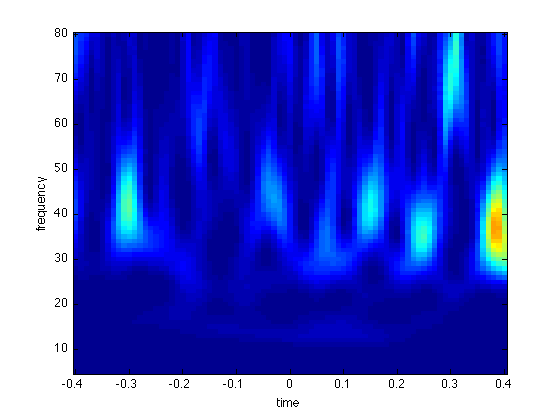
Figure: TFR of chan02 with large DC component (left) and chan01 without DC component (right) after ft_freqanalysis without demeaning
cfg.polyremoval
Note, in the above code cfg.polyremoval = -1. This option has been introduced in July 2011 (see this email thread). The default behavior is cfg.polyremoval = 0, which means that the zero-order polynomial is removed, which is equal to demeaning. So if you’re just using the default in ft_freqanalysis, your data will be automatically demeaned (you don’t have to do in separately in ft_preprocessing), aiming to avoid these surprising effects. A value of -1 is NOT the default behavior, because it will lead to no demeaning whatsoever, and therefore shows the strange behavior. Also see Why does my TFR look strange (part II)? for info on detrending (is first-order polynomial removal).