Time-frequency analysis using Hanning window, multitapers and wavelets
Introduction
In this tutorial you can find information about the time-frequency analysis of a single subject’s MEG data using a Hanning window, multitapers and wavelets. This tutorial also shows how to visualize the results.
Here, we will work on the MEG-language dataset, you can click here for details on the dataset. This tutorial is a continuation from the preprocessing tutorials. We will begin by repeating the code used to select the trials and preprocess the data as described in the earlier tutorials (trigger-based trial selection, artifact rejection). We assume that the reader already knows how to do the preprocessing in FieldTrip.
There is no information in this tutorial about how to compare conditions, how to grandaverage the results across subjects or how to do statistical analysis on the time-frequency data. Some of these issues are covered in other tutorials (see the summary and suggested further reading section).
This tutorial contains hands-on material that we use for the MEG/EEG toolkit course and it is complemented by this lecture.
Background
Oscillatory components contained in the ongoing EEG or MEG signal often show power changes relative to experimental events. These signals are not necessarily phase-locked to the event and will not be represented in event-related fields and potentials (Tallon-Baudry and Bertrand (1999)). The goal of this section is to compute and visualize event-related changes by calculating time-frequency representations (TFRs) of power. This will be done using analysis based on Fourier analysis and wavelets. The Fourier analysis will include the application of multitapers (Mitra and Pesaran (1999), Percival and Walden (1993)) which allow a better control of time and frequency smoothing.
Calculating time-frequency representations of power is done using a sliding time window. This can be done according to two principles: either the time window has a fixed length independent of frequency, or the time window decreases in length with increased frequency. For each time window the power is calculated. Prior to calculating the power one or more tapers are multiplied with the data. The aim of the tapers is to reduce spectral leakage and control the frequency smoothing.
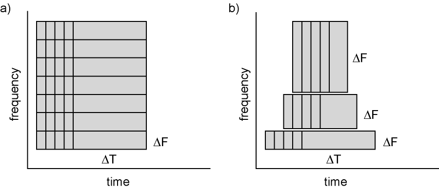
Figure: Time and frequency smoothing. (a) For a fixed length time window the time and frequency smoothing remains fixed. (b) For time windows that decrease with frequency, the temporal smoothing decreases and the frequency smoothing increases.
If you want to know more about tapers/ window functions you can have a look at this Wikipedia site. Note that Hann window is another name for Hanning window used in this tutorial. There is also a Wikipedia site about multitapers, to take a look at it click here.
Procedure
To calculate the time-frequency analysis for the example dataset we will perform the following steps:
- Read the data into MATLAB using ft_definetrial and ft_preprocessing
- Seperate the trials from each condition using ft_selectdata
- Compute the power values for each frequency bin and each time bin using the function ft_freqanalysis
- Visualize the results. This can be done by creating time-frequency plots for one (ft_singleplotTFR) or several channels (ft_multiplotTFR), or by creating a topographic plot for a specified time- and frequency interval (ft_topoplotTFR).
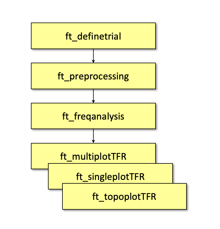
Figure: Schematic overview of the steps in time-frequency analysis
In this tutorial, procedures of 4 types of time-frequency analysis will be shown. You can see each of them under the titles: Time-frequency analysis I, II … and so on. If you are interested in a detailed description about how to visualize the results, look at the visualization part.
Preprocessing
The first step is to read the data using the function ft_preprocessing. With the aim to reduce boundary effects occurring at the start and the end of the trials, it is recommended to read larger time intervals than the time period of interest. In this example, the time of interest is from -0.5 s to 1.5 s (t = 0 s defines the time of stimulus); however, the script reads the data from -1.0 s to 2.0 s.
Reading in the data
We will now read and preprocess the data. If you would like to continue directly with the already preprocessed data, you can download dataFIC.mat. Load the data into MATLAB with the command load dataFIC and skip to Time-frequency analysis I.
Otherwise run the following code:
The ft_definetrial and ft_preprocessing functions require the original MEG dataset, which is available here
Do the trial definition for the all conditions together:
cfg                         = [];
cfg.dataset                 = 'Subject01.ds';
cfg.trialfun                = 'ft_trialfun_general'; % this is the default
cfg.trialdef.eventtype      = 'backpanel trigger';
cfg.trialdef.eventvalue     = [3 5 9]; % the values of the stimulus trigger for the three conditions
% 3 = fully incongruent (FIC), 5 = initially congruent (IC), 9 = fully congruent (FC)
cfg.trialdef.prestim        = 1; % in seconds
cfg.trialdef.poststim       = 2; % in seconds

cfg = ft_definetrial(cfg);
Cleaning
% remove the trials that have artifacts from the trl
cfg.trl([2, 5, 6, 8, 9, 10, 12, 39, 43, 46, 49, 52, 58, 84, 102, 107, 114, 115, 116, 119, 121, 123, 126, 127, 128, 133, 137, 143, 144, 147, 149, 158, 181, 229, 230, 233, 241, 243, 245, 250, 254, 260],:) = [];


% preprocess the data
cfg.channel   = {'MEG', '-MLP31', '-MLO12'};        % read all MEG channels except MLP31 and MLO12
cfg.demean    = 'yes';                              % do baseline correction with the complete trial

data_all = ft_preprocessing(cfg);
These data have been cleaned from artifacts by removing several trials and two sensors; see the visual artifact rejection tutorial.
We select one of the conditions from the original dataset for time-frequency analysis:
cfg = [];
cfg.trials = data_all.trialinfo == 3;
dataFIC = ft_redefinetrial(cfg, data_all);
Subsequently you can save the data to disk.
save dataFIC dataFIC
Time-frequency analysis I
Hanning taper, fixed window length
Here, we will describe how to calculate time frequency representations using Hanning tapers. When choosing for a fixed window length procedure the frequency resolution is defined according to the length of the time window (delta T). The frequency resolution (delta f in figure 1) = 1/length of time window in sec (delta T in figure 1). Thus a 500 ms time window results in a 2 Hz frequency resolution (1/0.5 sec= 2 Hz) meaning that power can be calculated for 2 Hz, 4 Hz, 6 Hz etc. An integer number of cycles must fit in the time window.
Ft_freqanalysis requires preprocessed data (see above), which can also be downloaded here.
load dataFIC
In the following example a time window with length 500 ms is applied.
cfg              = [];
cfg.output       = 'pow';
cfg.channel      = 'MEG';
cfg.method       = 'mtmconvol';
cfg.taper        = 'hanning';
cfg.foi          = 2:2:30;                         % analysis 2 to 30 Hz in steps of 2 Hz
cfg.t_ftimwin    = ones(length(cfg.foi),1).*0.5;   % length of time window = 0.5 sec
cfg.toi          = -0.5:0.05:1.5;                  % time window "slides" from -0.5 to 1.5 sec in steps of 0.05 sec (50 ms)
TFRhann = ft_freqanalysis(cfg, dataFIC);
Regardless of the method used for calculating the TFR, the output format is identical. It is a structure with the following fields:
TFRhann =

        label: {149x1 cell}                % Channel names
       dimord: 'chan_freq_time'            % Dimensions contained in powspctrm, channels X frequencies X time
         freq: [2 4 6 8 10 12 14 16 18 20 22 24 26 28 30]  % Array of frequencies of interest (the elements of freq may be different from your cfg.foi input depending on your trial length)
         time: [1x41 double]               % Array of time points considered
    powspctrm: [149x15x41 double]          % 3-D matrix containing the power values
         elec: [1x1 struct]                % Electrode positions etc
         grad: [1x1 struct]                % Gradiometer positions etc
          cfg: [1x1 struct]                % Settings used in computing this frequency decomposition
The field TFRhann.powspctrm contains the temporal evolution of the raw power values for each specified frequency.
If you specify frequencies in cfg.foi of which no integer number of cycles fit into you time window (cfg.t_ftimwin), FieldTrip doesn’t always give an error and the output will contain these frequencies. For example, try using cfg.foi = 1:1:30 with the 500 ms time window. Note that the uneven frequencies cannot be interpreted. So you should always think critically about your time and frequency resolution.
Visualization
This part of the tutorial shows how to visualize the results of any type of time-frequency analysis.
To visualize the event-related power changes, a normalization with respect to a baseline interval will be performed. There are two possibilities for normalizing:
- Subtracting, for each frequency, the average power in a baseline interval from all other power values. This gives, for each frequency, the absolute change in power with respect to the baseline interval.
- Expressing, for each frequency, the raw power values as the relative increase or decrease with respect to the power in the baseline interval. This means active period/baseline. Note that the relative baseline is expressed as a ratio; i.e. no change is represented by 1.
There are three ways of graphically representing the data: 1) time-frequency plots of all channels, in a quasi-topographical layout, 2) time-frequency plot of an individual channel (or average of several channels), 3) topographical 2-D map of the power changes in a specified time-frequency interval.
To plot the TFRs from all the sensors use the function ft_multiplotTFR. Settings can be adjusted in the cfg structure. For example:
cfg = [];
cfg.baseline     = [-0.5 -0.1];
cfg.baselinetype = 'absolute';
cfg.zlim         = [-2.5e-27 2.5e-27];
cfg.showlabels   = 'yes';
cfg.layout       = 'CTF151_helmet.mat';
figure
ft_multiplotTFR(cfg, TFRhann);
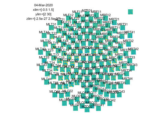
Figure: Time-frequency representations calculated using ft_freqanalysis. Plotting was done with ft_multiplotTFR)
Note that using the options cfg.baseline and cfg.baselinetype results in baseline correction of the data. Baseline correction can also be applied directly by calling ft_freqbaseline. Moreover, you can combine the various visualization options/functions interactively to explore your data. Currently, this is the default plotting behavior because the configuration option cfg.interactive=’yes’ is activated unless you explicitly select cfg.interactive=’no’ before calling ft_multiplotTFR to deactivate it. See also the plotting tutorial for more details.
An interesting effect seems to be present in the TFR of sensor MRC15. To make a plot of a single channel use the function ft_singleplotTFR.
cfg = [];
cfg.baseline     = [-0.5 -0.1];
cfg.baselinetype = 'absolute';
cfg.maskstyle    = 'saturation';
cfg.zlim         = [-2.5e-27 2.5e-27];
cfg.channel      = 'MRC15';
cfg.layout       = 'CTF151_helmet.mat';
figure
ft_singleplotTFR(cfg, TFRhann);
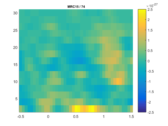
Figure: The time-frequency representation of a single sensor obtained using ft_singleplotTFR
If you see artifacts in your figure, see this question.
From the previous figure you can see that there is an increase in power around 15-20 Hz in the time interval 0.9 to 1.3 s after stimulus onset. To show the topography of the beta increase use the function ft_topoplotTFR.
cfg = [];
cfg.baseline     = [-0.5 -0.1];
cfg.baselinetype = 'absolute';
cfg.xlim         = [0.9 1.3];
cfg.zlim         = [-1e-27 1e-27];
cfg.ylim         = [15 20];
cfg.marker       = 'on';
cfg.layout       = 'CTF151_helmet.mat';
cfg.colorbar     = 'yes';
figure
ft_topoplotTFR(cfg, TFRhann);
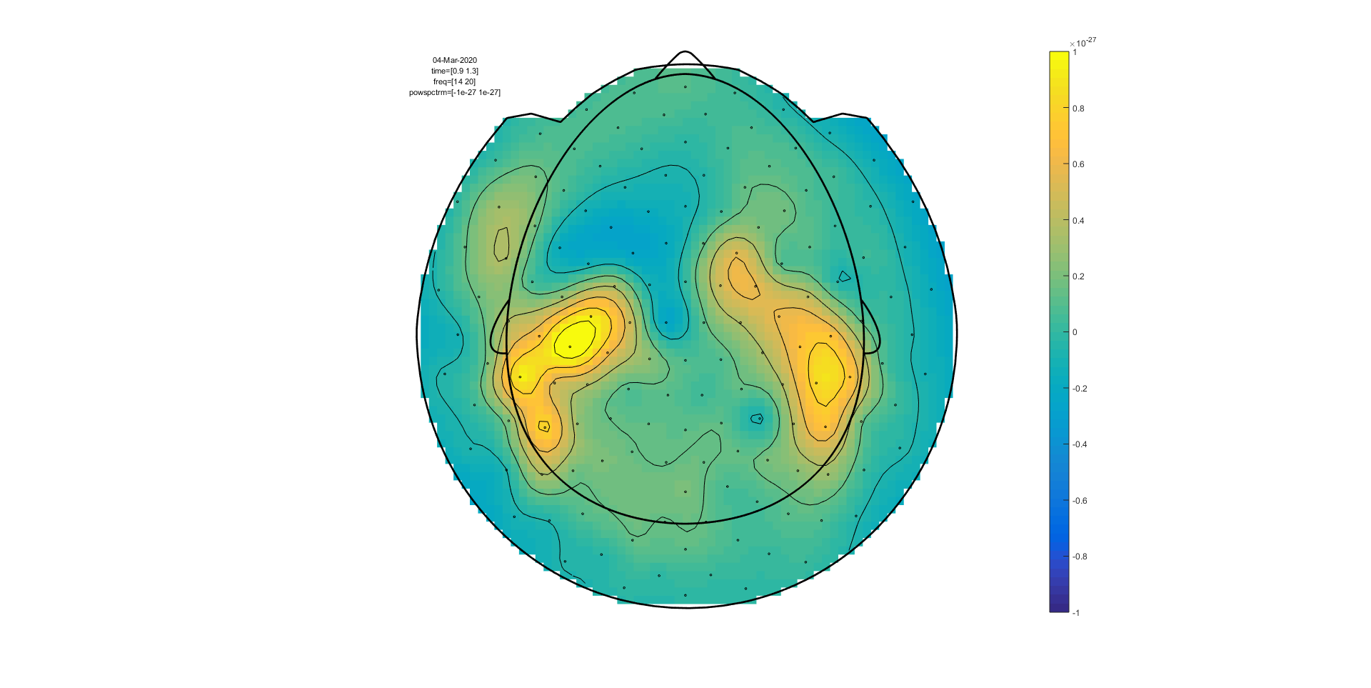
Figure: A topographic representation of the time-frequency representations (15 - 20 Hz, 0.9 - 1.3 s post stimulus) obtained using ft_topoplotTFR
Exercise 1
Plot the power with respect to a relative baseline (hint: use cfg.zlim=[0 3.0] and use the cfg.baselinetype option)
How are the responses different? Discuss the assumptions behind choosing a relative or absolute baseline
Exercise 2
Plot the TFR of sensor MLC24. How do you account for the increased power at ~300 ms (hint: compare to ERFs)?
Time-frequency analysis II
Hanning taper, frequency dependent window length
It is also possible to calculate the TFRs with respect to a time window that varies with frequency. Typically the time window gets shorter with an increase in frequency. The main advantage of this approach is that the temporal smoothing decreases with higher frequencies, leading to increased sensitivity to short-lived effects. However, an increased temporal resolution is at the expense of frequency resolution (why?). We will here show how to perform a frequency-dependent time-window analysis, using a sliding window Hanning taper based approach. The approach is very similar to wavelet analysis. A wavelet analysis performed with a Morlet wavelet mainly differs by applying a Gaussian shaped taper (see Time-frequency analysis IV).
The analysis is best done by first selecting the numbers of cycles per time window which will be the same for all frequencies. For instance if the number of cycles per window is 7, the time window is 1000 ms for 7 Hz (1/7 x 7 cycles); 700 ms for 10 Hz (1/10 x 7 cycles) and 350 ms for 20 Hz (1/20 x 7 cycles). The frequency can be chosen arbitrarily - however; too fine a frequency resolution is just going to increase the redundancy rather than providing new information.
Below is the configuration for a 7-cycle time window. The calculation is only done for one sensor (MRC15) but it can of course be extended to all sensors.
cfg              = [];
cfg.output       = 'pow';
cfg.channel      = 'MRC15';
cfg.method       = 'mtmconvol';
cfg.taper        = 'hanning';
cfg.foi          = 2:1:30;
cfg.t_ftimwin    = 7./cfg.foi;  % 7 cycles per time window
cfg.toi          = -0.5:0.05:1.5;
TFRhann7 = ft_freqanalysis(cfg, dataFIC);
To plot the result use ft_singleplotTFR:
cfg              = [];
cfg.baseline     = [-0.5 -0.1];
cfg.baselinetype = 'absolute';
cfg.maskstyle    = 'saturation';
cfg.zlim         = [-2e-27 2e-27];
cfg.channel      = 'MRC15';
cfg.interactive  = 'no';
cfg.layout       = 'CTF151_helmet.mat';
figure
ft_singleplotTFR(cfg, TFRhann7);
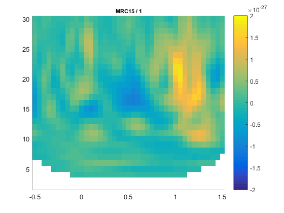
Figure: A time-frequency representation of channel MRC15 obtained using ft_singleplotTFR
If you see artifacts in your figure, see this FAQ.
Boundary effects Note the boundary effects, in particular for the lower frequency bins, i.e. the blue (or white) region in the time frequency plane. Within this region, no power values are calculated. The reason for this is that for the corresponding time points, the requested timewindow is not entirely filled with data. For example for 2 Hz the time window has a length of 3.5 s (7 cycles for 2 cycles/s = 3.5 s), this does not fit in the 3 sec window that is preprocessed and therefore there is no data point here. For 5 Hz the window has a length of 1.4 s (7 cycles for 5 cycles/s = 1.4 s). We preprocessed data between t = -1 sec and t = 2 sec so the first power value is assigned to t= -0.3 (since -1 + (0.5 * 1.4) = -0.3). Because of these boundary effects it is important to apply ft_freqanalysis to a larger time window to get all the time frequency points for your time window of interest. This requires some thinking ahead when designing your experiment, because inclusion of data from epochs-of-non-interest might contaminate your data with artifacts or other unwanted data features (e.g., stimulus-offset related rebounds).
If you would like to learn more about plotting of time-frequency representations, please see the visualization section.
Exercise 3
Adjust the length of the time-window and thereby degree of smoothing. Use ft_singleplotTFR to show the results. Discuss the consequences of changing these setting.
4 cycles per time window:
cfg              = [];
cfg.output       = 'pow';
cfg.channel      = 'MRC15';
cfg.method       = 'mtmconvol';
cfg.taper        = 'hanning';
cfg.foi          = 2:1:30;
cfg.t_ftimwin    = 4./cfg.foi;
cfg.toi          = -0.5:0.05:1.5;
TFRhann4 = ft_freqanalysis(cfg, dataFIC);
5 cycles per time window:
cfg.t_ftimwin    = 5./cfg.foi;
TFRhann5 = ft_freqanalysis(cfg, dataFIC);
10 cycles per time window:
cfg.t_ftimwin    = 10./cfg.foi;
TFRhann10 = ft_freqanalysis(cfg, dataFIC);
Time-frequency analysis III
Multitapers
Multitapers are typically used in order to achieve better control over the frequency smoothing. More tapers for a given time window will result in stronger smoothing. For frequencies above 30 Hz, smoothing has been shown to be advantageous, increasing sensitivity thanks to reduced variance in the estimates despite reduced effective spectral resolution. Oscillatory gamma activity (30-100 Hz) is quite broad band and thus analysis of this signal component benefits from multitapering, which trades spectral resolution against increased sensitivity. For signals lower than 30 Hz it is recommend to use only a single taper, e.g., a Hanning taper as shown above (beware that in the example below multitapers are used to analyze low frequencies because there are no effects in the gamma band in this dataset).
Time-frequency analysis based on multitapers can be performed by the function ft_freqanalysis. The function uses a sliding time window for which the power is calculated for a given frequency. Prior to calculating the power by discrete Fourier transforms the data are ‘tapered’. Several orthogonal tapers might be used for each time window. The power is calculated for each tapered data segment and then combined. In the example below we apply a time window which gradually becomes shorter for higher frequencies (similar to wavelet techniques). Note that this is not necessary, but up to the researcher to decide. The arguments for the chosen parameters are as follows:
- cfg.foi, the frequencies of interest, here from 1 Hz to 30 Hz in steps of 2 Hz. The step size could be decreased at the expense of computation time and redundancy.
- cfg.toi, the time-interval of interest. This vector determines the center times for the time windows for which the power values should be calculated. The setting cfg.toi = -0.5:0.05:1.5 results in power values from -0.5 to 1.5 s in steps of 50 ms. A finer time resolution will give redundant information and longer computation times, but a smoother graphical output.
- cfg.t_ftimwin is the length of the sliding time-window in seconds (= tw). We have chosen cfg.t_ftimwin = 5./cfg.foi, i.e. 5 cycles per time-window. When choosing this parameter it is important that a full number of cycles fit within the time-window for a given frequency.
- cfg.tapsmofrq determines the width of frequency smoothing in Hz (= fw). We have chosen cfg.tapsmofrq = cfg.foi*0.4, i.e. the smoothing will increase with frequency. Specifying larger values will result in more frequency smoothing. For less smoothing you can specify smaller values, however, the following relation determined by the Shannon number must hold (see Percival and Walden (1993)):
K = 2*tw*fw-1, where K is required to be larger than 0. K is the number of tapers applied; the more, the greater the smoothing.
These settings result in the following characteristics as a function of the frequencies of interest:

Figure: a) The characteristics of the TFRs settings using multitapers in terms of time and frequency resolution of the settings applied in the example. b) Examples of the time-frequency tiles resulting from the settings.
cfg = [];
cfg.output     = 'pow';
cfg.channel    = 'MEG';
cfg.method     = 'mtmconvol';
cfg.foi        = 1:2:30;
cfg.t_ftimwin  = 5./cfg.foi;
cfg.tapsmofrq  = 0.4 *cfg.foi;
cfg.toi        = -0.5:0.05:1.5;
TFRmult = ft_freqanalysis(cfg, dataFIC);
Plot the result
cfg = [];
cfg.baseline     = [-0.5 -0.1];
cfg.baselinetype = 'absolute';
cfg.zlim         = [-2e-27 2e-27];
cfg.showlabels   = 'yes';
cfg.layout       = 'CTF151_helmet.mat';
cfg.colorbar     = 'yes';
figure
ft_multiplotTFR(cfg, TFRmult)
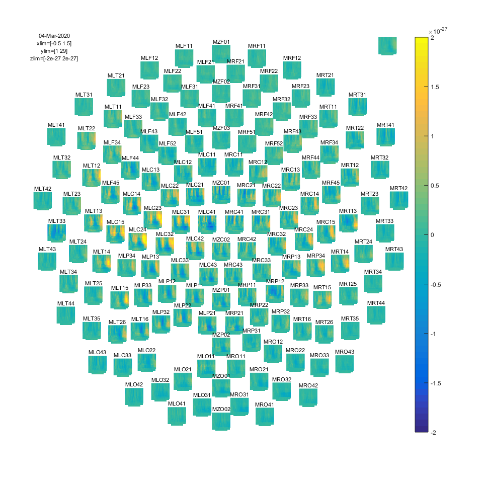
Figure: Time-frequency representations of power calculated using multitapers.
If you would like to learn more about plotting of time-frequency representations, please see the visualization section.
Time-frequency analysis IV
Morlet wavelets
An alternative to calculating TFRs with the multitaper method is to use Morlet wavelets. The approach is equivalent to calculating TFRs with time windows that depend on frequency using a taper with a Gaussian shape. The commands below illustrate how to do this. One crucial parameter to set is cfg.width. It determines the width of the wavelets in number of cycles. Making the value smaller will increase the temporal resolution at the expense of frequency resolution and vice versa. The spectral bandwidth at a given frequency F is equal to F/width*2 (so, at 30 Hz and a width of 7, the spectral bandwidth is 30/7*2 = 8.6 Hz) while the wavelet duration is equal to width/F/pi (in this case, 7/30/pi = 0.074s = 74ms) (Tallon-Baudry and Bertrand (1999)).
Calculate TFRs using Morlet wavelet
cfg = [];
cfg.channel    = 'MEG';
cfg.method     = 'wavelet';
cfg.width      = 7;
cfg.output     = 'pow';
cfg.foi        = 1:2:30;
cfg.toi        = -0.5:0.05:1.5;
TFRwave = ft_freqanalysis(cfg, dataFIC);
Plot the result
cfg = [];
cfg.baseline     = [-0.5 -0.1];
cfg.baselinetype = 'absolute';
cfg.zlim         = [-2e-25 2e-25];
cfg.showlabels   = 'yes';
cfg.layout       = 'CTF151_helmet.mat';
cfg.colorbar     = 'yes';
figure
ft_multiplotTFR(cfg, TFRwave)
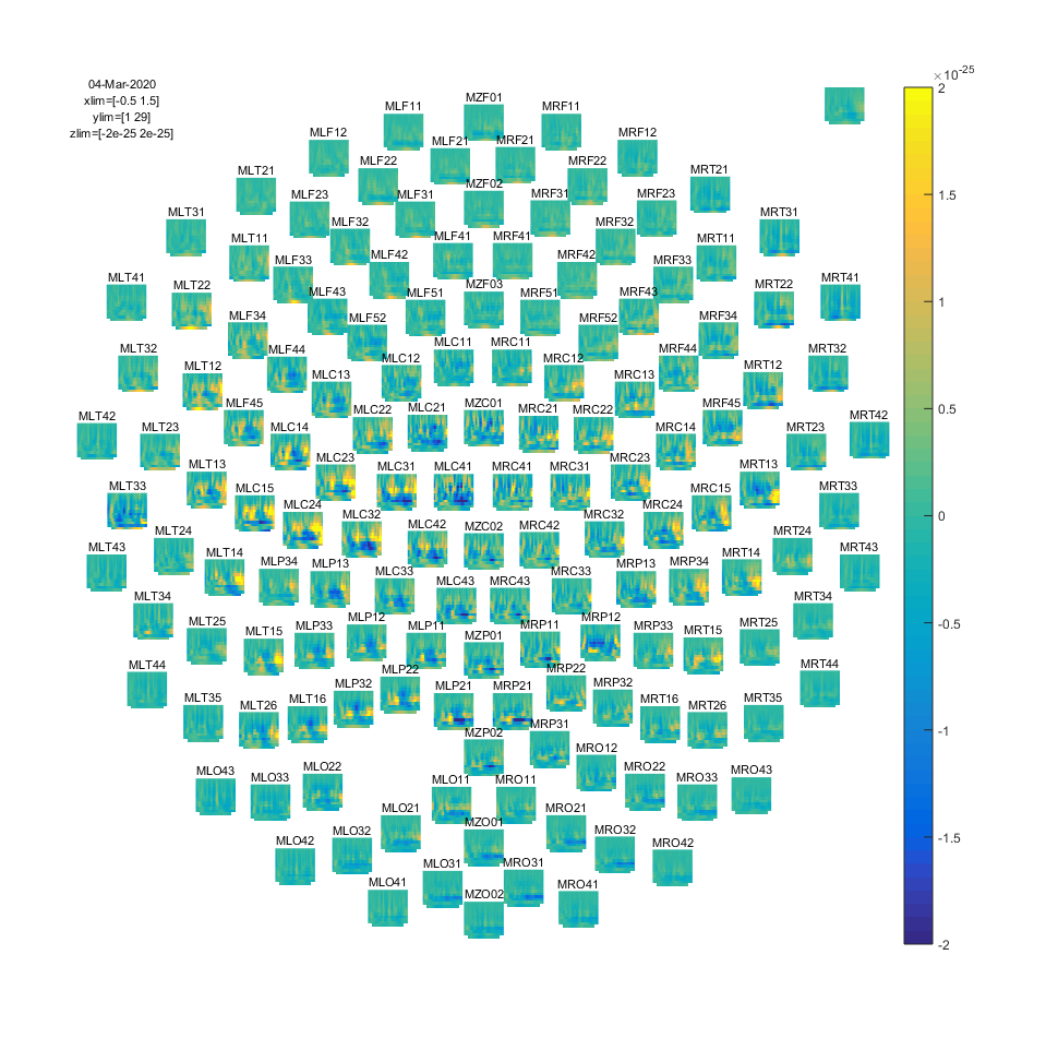
Figure: Time-frequency representations of power calculated using Morlet wavelets.
Exercise 4:
Adjust cfg.width and see how the TFRs change.
If you would like to learn more about plotting of time-frequency representations, please see visualization.
Summary and suggested further reading
This tutorial showed how to do time-frequency analysis on a single’s subject MEG data and how to plot the time-frequency representations. There were 4 methods shown for calculating time-frequency representations and 3 functions for plotting the results.
After having finished this tutorial on time-frequency analysis, you can continue with the Localizing oscillatory sources using beamformer techniques tutorial if you are interested in the source-localization of the power changes or the Cluster-based permutation tests on time-frequency data tutorial if you are interested how to do statistics on the time-frequency representations.
Frequently asked question
- Does it make sense to subtract the ERP prior to time frequency analysis, to distinguish evoked from induced power?
- How can I do time-frequency analysis on continuous data?
- How can I test whether a behavioral measure is phasic?
- In what way can frequency domain data be represented in FieldTrip?
- How does MTMCONVOL work?
- What are the differences between the old and the new implementation of 'mtmconvol' in ft_freqanalyis?
- What are the differences between the old and the new implementation of 'mtmftt' in ft_freqanalyis?
- What are the differences between the old and the new implementation of 'wavelet' (formerly 'wltconvol') in ft_freqanalyis?
- What convention is used to define absolute phase in 'mtmconvol', 'wavelet' and 'mtmfft'?
- What does "padding not sufficient for requested frequency resolution" mean?
- What kind of filters can I apply to my data?
- Why am I not getting integer frequencies?
- Why does my output.freq not match my cfg.foi when using 'mtmconvol' in ft_freqanalyis?
- Why does my output.freq not match my cfg.foi when using 'mtmfft' in ft_freqanalyis
- Why does my output.freq not match my cfg.foi when using 'wavelet' (formerly 'wltconvol') in ft_freqanalyis?
- Why does my TFR contain NaNs?
- Why does my TFR look strange (part I, demeaning)?
- Why does my TFR look strange (part II, detrending)?
- Why is the largest peak in the spectrum at the frequency which is 1/segment length?
Example script
- Apply non-parametric statistics with clustering on TFRs of power that were computed with BESA
- Effect of SNR on Coherence
- Common filters in beamforming
- Conditional Granger causality in the frequency domain
- Correlation analysis of fMRI data
- Cross-frequency analysis
- Effects of tapering for power estimates
- Fourier analysis of neuronal oscillations and synchronization
- Simulate an oscillatory signal with phase resetting
- Analyze Steady-State Visual Evoked Potentials (SSVEPs)