Introduction to the FieldTrip toolbox
Introduction
This tutorial will give you an introduction into how to use FieldTrip with MATLAB and how to make an analysis protocol. You will read a few examples of analysis protocols of EEG/MEG data analysis. This introduction, however, does not give detailed information about each analysis step. You will find those in other tutorials. You will find also useful information about how to use FieldTrip in the walkthrough.
This short tutorial introduces the design of the FieldTrip toolbox. If you have some more time, you can watch a more elaborate introduction in this lecture.
Background
When performing EEG/MEG experiments, the aim is to gain insight into the functioning of the brain while it is engaged in certain activities. When analyzing EEG/MEG data, we hope to identify the aspects of the data that relate to the experimental question. This means that we seek to reduce the data to interpretable concepts or statements regarding hypotheses underlying the experiment. The successful analysis of EEG/MEG data does not only depend on acquiring good quality data, but also on incorporating the researcher’s knowledge and assumptions into the analysis protocol.
The analysis protocol includes tools and/or algorithms used, and how they are used. The knowledge or assumptions incorporated by the researcher in the protocol might be
- At a certain time after the presentation of a stimulus, the brain will process the stimulus.
- The brain will process repeated stimuli similarly.
- Electrical activity generated by the neurons in the brain has certain properties that distinguish it from artifacts, such as amplitude (eye movements result in much larger scalp potentials) or distribution (signals originating from the brain are picked up simultaneously by multiple neighboring electrodes).
- The scalp distribution of the EEG/MEG depends on the location of the underlying activity.
- Oscillatory activity is produced by certain brain regions.
These tools can be combined in an analysis protocol that for example looks like Figure 1.
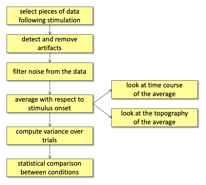
Figure: Analysis protocol for Event-Related Potentials (ERPs).
We will use the FieldTrip toolbox for EEG/MEG analysis that is developed within the Donders Centre for Cognitive Neuroimaging (DCCN). This software consists of a set of MATLAB functions (a toolbox) that implement the different steps. Each of the FieldTrip functions implements one tool, and by linking them you can perform a complete analysis.
The FieldTrip toolbox
The FieldTrip toolbox is not a program with a user interface where you can click around in, but rather a collection of functions. The functions can be grouped into a few major categories:
- Functions for preprocessing, reading and converting data (e.g., ft_preprocessing)
- Functions for analyzing event-related fields or potentials (ERF/ERP) (e.g., ft_timelockanalysis)
- Functions for frequency and time-frequency analysis (e.g., ft_freqanalysis)
- Functions for source analysis (e.g., ft_sourceanalysis)
- Functions for statistical analysis (e.g., ft_timelockstatistics)
- Functions for plotting and displaying the data (e.g., ft_multiplotER)
The full list of functions can be found here. Each of the functions of the toolbox takes as input the (intermediate) data that was produced by the previous function.
There is a difference between high- and low-level functions. The high-level functions are the ones that are used by the user, while the low-level functions are automatically called by the higher level functions. The user does not have to be aware of the low-level functions. The toolbox is continuously being developed and extended. Therefore, it is important that you start your analysis in the newest version of FieldTrip.
In some cases, FieldTrip is working together with external toolboxes or programs, like SPM, OpenMEEG and FreeSurfer. Some of the toolboxes are included in the default FieldTrip release, some of them have to be downloaded from the internet. You can read more about the external toolboxes here.
Using the toolbox and MATLAB
Each FieldTrip function implements a specific algorithm, for which specific parameters can be specified. These parameters on how the function behaves is passed as a configuration structure. Where applicable, the configuration parameters will have sensible defaults. The most convenient way of specifying the configuration is by typing it into a script in the MATLAB editor and copy-and-pasting that into the MATLAB command-line window. The configuration for ft_definetrial (for ctf data that is recorded in epochs) might look like this:
cfg1                         = [];
cfg1.dataset                 = 'Subject01.ds';
cfg1.trialdef.eventtype      = 'backpanel trigger';
cfg1.trialdef.eventvalue     = 3; % the value of the stimulus trigger for fully incongruent (FIC).
cfg1.trialdef.prestim        = 1;
cfg1.trialdef.poststim       = 2;
The functions in the FieldTrip toolbox are executed with the configuration structure (“cfg”) and in most cases with a data structure as inputs
Example
cfg1         = ft_definetrial(cfg1);
dataPrepro   = ft_preprocessing(cfg1);

cfg2         = [];
dataTimelock = ft_timelockanalysis(cfg2,dataPrepro);
Please note that each FieldTrip function has its own configuration structure and you should not mix them, except for a few functions that add something to the configuration structure (ft_definetrial and the artifact detection functions).
The help included in each function will explain the configurable settings and how they should be specified. In MATLAB, you can get help for a specific function by typing
help <functionname>
e.g.
help ft_preprocessing
How to make analysis protocols for different types of analysis using the FieldTrip toolbox can be found in the tutorials at this website.
Executing FieldTrip commands from MATLAB
FieldTrip is composed of a collection of scripts running in MATLAB. The toolbox is platform independent (i.e. can run under Linux, macOS and Windows). To start MATLAB on Linux at the DCC
matlab2022a # or use another version number, e.g., matlab2018b
It is now possible to execute the MATLAB scripts by copying/pasting the relevant text from the tutorials (To copy from a Window browser to MATLAB running under Linux from X-Win32, use the mouse to highlight the text in the browser and press crtl-c. Then use ctrl-v or the middle mouse button to paste in MATLAB).
Make sure that the path is set correctly to the directory of the FieldTrip toolbox and the data. For the tutorials it is recommend to ‘cd’ to the directory where the data are. Look at this FAQ for more information on how to correctly set your path for FieldTrip.
Making an analysis protocol
When you are using FieldTrip, your analysis protocol is the MATLAB script, in which you call the different FieldTrip functions. Such a script (or set of scripts) can be considered as an analysis protocol, since in them you are defining all the steps that you are taking during the analysis. For most of the analysis steps, you will be able to use a function from the FieldTrip toolbox, but sometimes you also will want to include your own MATLAB code in the script.
In the next section, you will see how the protocol of the ERP example looks using FieldTrip. Some other standard analysis protocols are given also below. The figures indicate which functions you (probably) will use in the analysis, and give you a guideline in finding the documentation that you need.
ERP/ERF analysis
ERP/ERF analysis consists of preprocessing, averaging the data timelocked to the stimulus or response, optionally averaging over subjects and/or testing for significant effects and finally plotting the result.
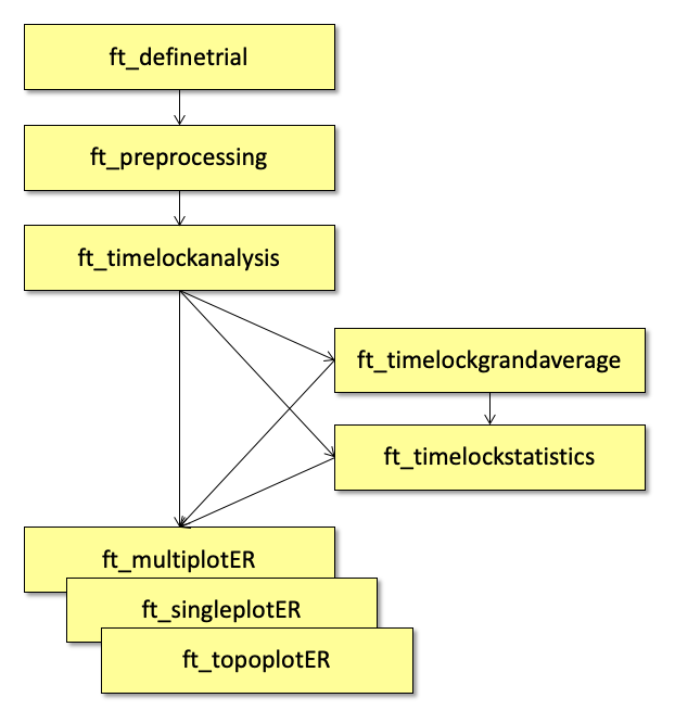
Figure: An example analysis protocol for Event-Related Potentials (ERPs) using the FieldTrip functions.
Frequency and time-frequency analysis
Frequency analysis consists of preprocessing, performing a Fourier or wavelet decomposition of the data, optionally averaging over subjects and/or testing for significant effects and finally plotting the result.
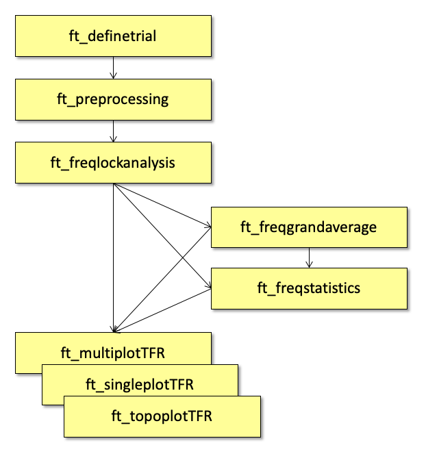
Figure: An example analysis protocol of (time-)frequency analysis in FieldTrip.
Beamformer source analysis
A schematic display of the analysis steps for source reconstruction using a beamformer approach is given below. Prior to any source reconstruction, you should have performed a complete timelock or frequency analysis of the data at the channel level.
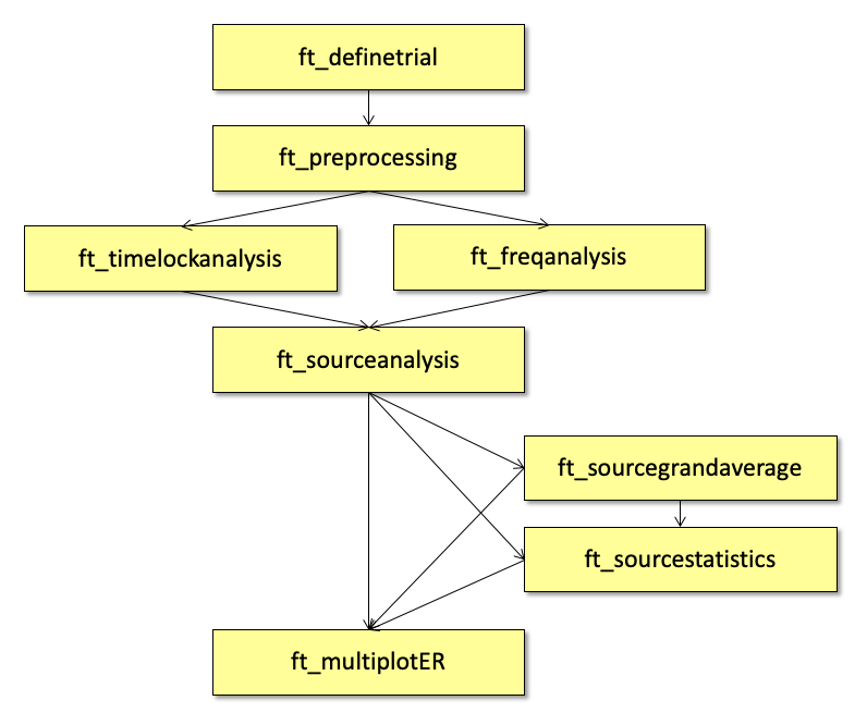
Figure: An example analysis protocol of the source analysis using beamforming in FieldTrip.
Source reconstruction for multiple subjects
If you do a source reconstruction of the data for multiple subjects, and if you use individual volume conduction models for your subjects (common for MEG), then the individual source reconstructions cannot immediately be averaged or used for statistical comparison. The anatomy of each subject is different (i.e. the shape and size of the brain), and the locations of the voxels (i.e. the dipoles) will also be different for each subject. Using the individual subject’s anatomical MRI, you can align all subjects to a template brain using a non-linear deformation. The same deformation can be applied to the functional data. Subsequently the subjects functional data can be compared.
The spatial normalisation towards a template brain is done in FieldTrip with the ft_volumenormalise function, which internally calls some low-level functions from the SPM2 toolbox. In general, it is also advisable to normalise your individual subject’s data to the SPM/MNI template brain.
Below you can see the protocol that you would use for averaging the source reconstruction over subjects and for group statistics on the source level. If the statistical test involves two conditions, then you should do the source normalisation in both conditions for all subjects and feed the two grandaveraged source reconstructions into ft_sourcestatistics.
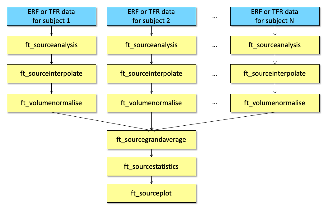
Figure: An example analysis protocol of source reconstruction for multiple subjects in FieldTrip.
Summary and suggested further reading
On this page we gave a short introduction about the FieldTrip toolbox and about how to use that in MATLAB. We have shown also some examples of analysis protocols.
If you would like to read further about the FieldTrip function, you can continue with the Preprocessing tutorial. If you would like to have an introduction about scripting in MATLAB, it is suggested that you continue with the tutorial:scripting tutorial. If you are new to MATLAB or EEG/MEG analysis, you can take a look in References to review papers and teaching material.
When you have more questions about the topic of any tutorial, don’t forget to check the frequently asked questions and the example scripts.
Here are the frequently asked questions that are MATLAB specific:
- Can I prevent "external" toolboxes from being added to my MATLAB path?
- Can I use FieldTrip without MATLAB license?
- Which external toolboxes are used by FieldTrip?
- How can I compile the mex files on 64-bit Windows?
- How can I use my MacBook Pro for stimulus presentation in the MEG lab?
- How fast is the FieldTrip buffer for realtime data streaming?
- Installation and setting up the path
- MATLAB complains about a missing or invalid mex file, what should I do?
- MATLAB does not see the functions in the "private" directory
- Replacements for functions from MathWorks toolboxes
- What are the MATLAB requirements for using FieldTrip?
- MATLAB version 7.3 (2006b) crashes when I try to do ...
- MATLAB complains that mexmaci64 cannot be opened because the developer cannot be verified
- What are the MATLAB and external requirements?
- What are the different approaches I can take for distributed computing?
- Where can I find the dipoli command-line executable?
- Why are so many of the interesting functions in the private directories?
- Why are the fileio functions stateless, does the fseek not make them very slow?
Here are the example scripts that are MATLAB specific: