Event related averaging and planar gradient

In this tutorial we will continue working on the dataset described in the preprocessing tutorials. Below we will repeat code to select the trials and preprocess the data as described in the first tutorials ( trigger based trial selection, visual artifact rejection, automatic artifact rejection).

In this tutorial you can find information about how to compute an event related potential (ERP)/ event related field (ERF) and how to calculate the planar gradient.

ERP / ERF

When analyzing EEG or MEG signals, the aim is to investigate the modulation of the measured brain signals with respect to a certain event. However, due to intrinsic and extrinsic noise in the signals, which in single trials is often higher than the signal evoked by the brain; it is typically required to average data from several trials to increase the signal-to-noise ratio(SNR). One approach is to repeat a given event in your experiment and average the corresponding EEG/MEG signals. The assumption is that the noise is independent of the events and thus reduced when averaging, while the effect of interest is time-locked to the event. The approach results in ERPs and ERFs for respectively EEG and MEG. Timelock analysis can be used to calculate ERPs/ ERFs.

Planar gradient

The CTF MEG system has 151 first-order axial gradiometer sensors that measure the gradient of the magnetic field in the radial direction, i.e. orthogonal to the scalp. Often it is helpful to interpret the MEG fields after transforming the data to a planar gradient configuration, i.e. by computing the gradient tangential to the scalp. This representation of MEG data is comparable to the field measured by planar gradiometer sensors. One advantage of the planar gradient transformation is that the signal amplitude typically is largest directly above a source.

To calculate the event related field / potential for the example dataset we will perform the following steps:

• Read the data into Matlab using ft_definetrial and ft_preprocessing
• Compute the average over trials using the function ft_timelockanalysis
• Calculate the planar gradient with the functions ft_megplanar and ft_combineplanar
• Visualize the results. You can plot the ERF/ ERP of one channel with ft_singleplotER or several channels with ft_multiplotER, or by creating a topographic plot for a specified time- interval with ft_topoplotER
• Grandaverage and realignment (optional). When you have data from more than one subject you can make a grand average of the ERPs / ERFs with ft_timelockgrandaverage. ft_megrealign can be used to realign each subjects data to standard sensor positions before computing the grand average.

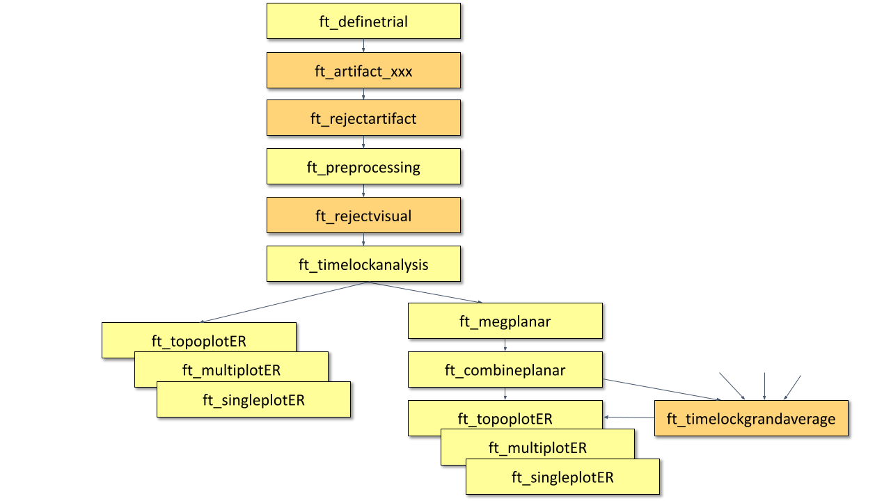
Figure 1; A schematic overview of the steps in averaging of event related fields

% find the interesting segments of data
cfg = [];                                           % empty configuration
cfg.dataset                 = 'Subject01.ds';       % name of CTF dataset  
cfg.trialdef.eventtype      = 'backpanel trigger';
cfg.trialdef.prestim        = 1;
cfg.trialdef.poststim       = 2;
cfg.trialdef.eventvalue     = 3;                    % trigger value for fully incongruent (FIC)
cfg = ft_definetrial(cfg);            

% remove the trials that have artifacts from the trl
cfg.trl([15, 36, 39, 42, 43, 49, 50, 81, 82, 84],:) = []; 

% preprocess the data
cfg.channel    = {'MEG', '-MLP31', '-MLO12'};        % read all MEG channels except MLP31 and MLO12
cfg.blc        = 'yes';
cfg.blcwindow  = [-0.2 0];
cfg.lpfilter   = 'yes';                              % apply lowpass filter
cfg.lpfreq     = 35;                                 % lowpass at 35 Hz.

dataFIC_LP = ft_preprocessing(cfg);                      

save dataFIC_LP dataFIC_LP

A note about padding: The padding parameter (cfg.padding) defines the duration to which the data in the trial will be padded (i.e. data-padded, not zero-padded). The padding is removed from the trial after filtering. Padding the data is beneficial, since the edge artifacts that are typically seen after filtering will be in the padding and not in the part of interest. Padding can also be relevant for DFT filtering of the 50Hz line noise artifact: long padding ensures a higher frequency resolution for the DFT filter, causing a narrower notch to be removed from the data. Padding can only be done on data that is stored in continuous format, therefore it is not used here.

If preprocessing was done as described dataFIC will have the following fields:

dataFIC_LP = 

      hdr: [1x1 struct]
    label: {149x1 cell}
    trial: {1x77 cell}
     time: {1x77 cell}
  fsample: 300
     grad: [1x1 struct]
      cfg: [1x1 struct]

Note that 'dataFIC_LP.label' has 149 in stead of 151 labels since channels MLP31 and MLO12 were excluded. 'dataFIC-LP.trial' has 77 in stead of 87 trials because 14 trials were rejected because of artifacts.

The most important fields are 'dataFIC_LP.trial' containing the individual trials and 'data.time' containing the time vector for each trial. To visualize the single trial data (trial 1) on one channel (channel 130) do the following:

plot(dataFIC_LP.time{1}, dataFIC_LP.trial{1}(130,:))

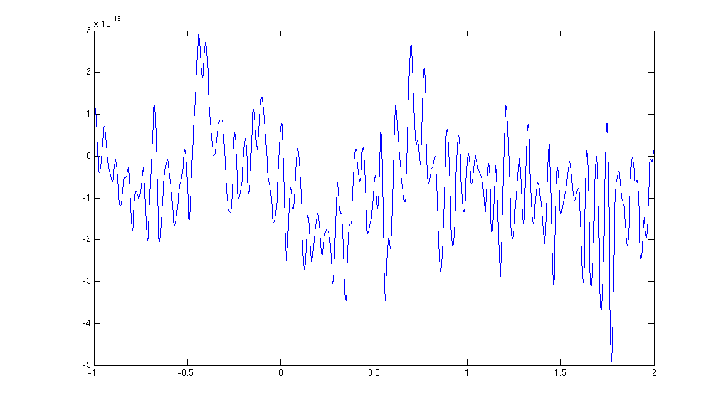
Figure 2; The MEG data from a single trial in a single sensor obtained after FT_PREPROCESSING

To perform the preprocessing for the initially congruent (IC) and fully congruent (FC) conditions write:

% find the interesting segments of data
cfg = [];                                           % empty configuration
cfg.dataset                 = 'Subject01.ds';       % name of CTF dataset  
cfg.trialdef.eventtype      = 'backpanel trigger';
cfg.trialdef.prestim        = 1;
cfg.trialdef.poststim       = 2;
cfg.trialdef.eventvalue     = 9;                    % trigger value for fully incongruent (FC)
cfg = ft_definetrial(cfg);            

% remove the trials that have artifacts from the trl
cfg.trl([2, 3, 4, 30, 39, 40, 41, 45, 46, 47, 51, 53, 59, 77, 85],:) = []; 

% preprocess the data
cfg.channel    = {'MEG', '-MLP31', '-MLO12'};       % read all MEG channels except MLP31 and MLO12
cfg.blc        = 'yes';
cfg.blcwindow  = [-0.2 0];
cfg.lpfilter   = 'yes';                              % apply lowpass filter
cfg.lpfreq     = 35;                                 % lowpass at 35 Hz.

dataFC_LP = ft_preprocessing(cfg);                      

save dataFC_LP dataFC_LP

% find the interesting segments of data
cfg = [];                                           % empty configuration
cfg.dataset                 = 'Subject01.ds';       % name of CTF dataset  
cfg.trialdef.eventtype      = 'backpanel trigger';
cfg.trialdef.prestim        = 1;
cfg.trialdef.poststim       = 2;
cfg.trialdef.eventvalue     = 5;                    % trigger value for initially congruent (IC)
cfg = ft_definetrial(cfg);            

% remove the trials that have artifacts from the trl
cfg.trl([1, 2, 3, 4, 14, 15, 16, 17, 20, 35, 39, 40, 47, 78, 79, 80, 86],:) = []; 

% preprocess the data
cfg.channel    = {'MEG', '-MLP31', '-MLO12'};        % read all MEG channels except MLP31 and MLO12
cfg.blc        = 'yes';
cfg.blcwindow  = [-0.2 0];
cfg.lpfilter   = 'yes';                              % apply lowpass filter
cfg.lpfreq     = 35;                                 % lowpass at 35 Hz.

dataIC_LP = ft_preprocessing(cfg);                      

save dataIC_LP dataIC_LP

The FieldTrip function ft_timelockanalysis makes averages of all the trials in a data structure.

The trials belonging to one condition will now be averaged with the onset of the stimulus time aligned to the zero-time point (the onset of the last word in the sentence). This is done with the function ft_timelockanalysis. The input to this procedure is the dataFIC structure generated by ft_preprocessing. No special settings are necessary here. Thus specify an empty configuration.

cfg = [];
avgFIC = ft_timelockanalysis(cfg, dataFIC_LP);
avgFC = ft_timelockanalysis(cfg, dataFC_LP);
avgIC = ft_timelockanalysis(cfg, dataIC_LP);

The output is the data structure avgFIC with the following fields:

avgFIC = 
         avg: [149x900 double]
         var: [149x900 double]
     fsample: 300
  numsamples: [77x1 double]
        time: [1x900 double]
         dof: [149x900 double]
       label: {149x1 cell}
      dimord: 'chan_time'
        grad: [1x1 struct]
         cfg: [1x1 struct]

An important field is avgFIC.avg, containing the average over all trials for each sensor.

Using the plot functions ft_multiplotER, ft_singleplotER and ft_topoplotER you can make plots of the average.

Use ft_multiplotER to plot all sensors in one figure:

cfg = [];
cfg.showlabels = 'yes'; 
cfg.fontsize = 6; 
cfg.layout = 'CTF151s.lay';
cfg.ylim = [-3e-13 3e-13];
ft_multiplotER(cfg, avgFIC); 

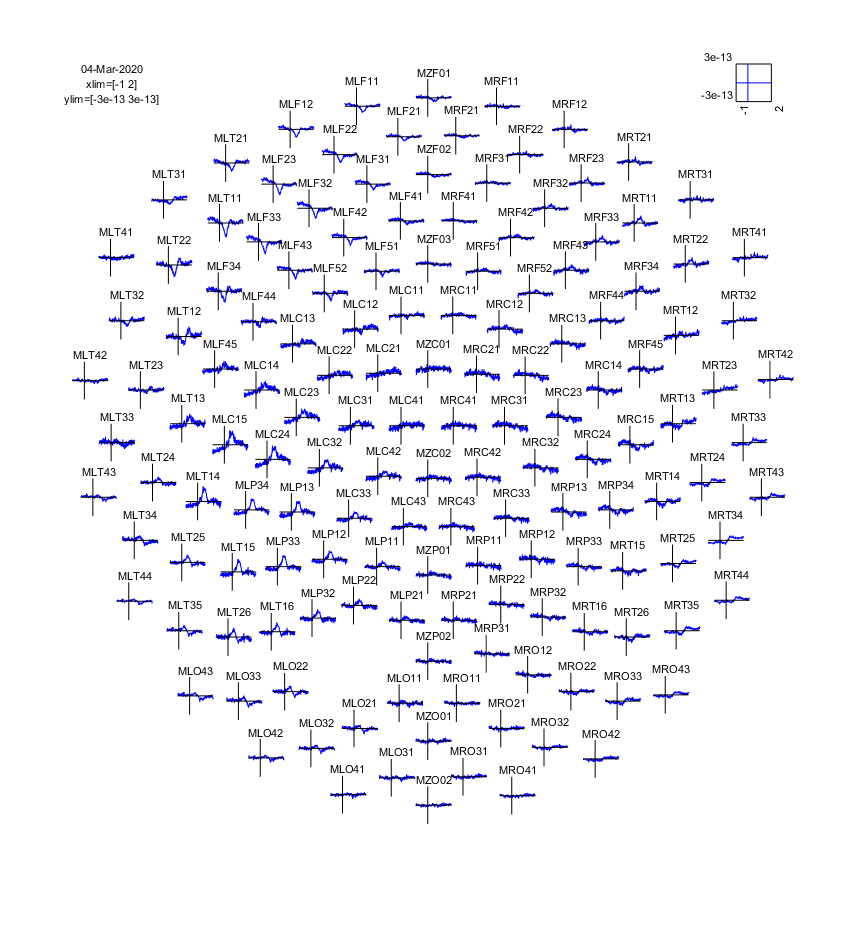
Figure 3; The event related fields plotted using ft_multiplotER. The event related fields were calculated using FT_PREPROCESSING followed by FT_TIMELOCKANALYSIS

This plots the event related fields for all sensors arranged topographically according to their position in the helmet. You can use the zoom button (magnifying glass) to enlarge parts of the figure. To plot all conditions list them as multiple variables:

cfg = [];
cfg.showlabels = 'no'; 
cfg.fontsize = 6; 
cfg.layout = 'CTF151s.lay';
cfg.baseline = [-0.2 0]; 
cfg.xlim = [-0.2 1.0]; 
cfg.ylim = [-3e-13 3e-13]; 
ft_multiplotER(cfg, avgFC, avgIC, avgFIC);

Figure 4; The event related fields for three conditions plotted simultaneously using ft_multiplotER

To plot one sensor data use ft_singleplotER and specify the name of the channel you are interested in, for instance MLC24:

cfg.xlim = [-0.2 1.0];
cfg.ylim = [-1e-13 3e-13];
cfg.channel = 'MLC24';
clf;
ft_singleplotER(cfg,avgFC, avgIC, avgFIC);

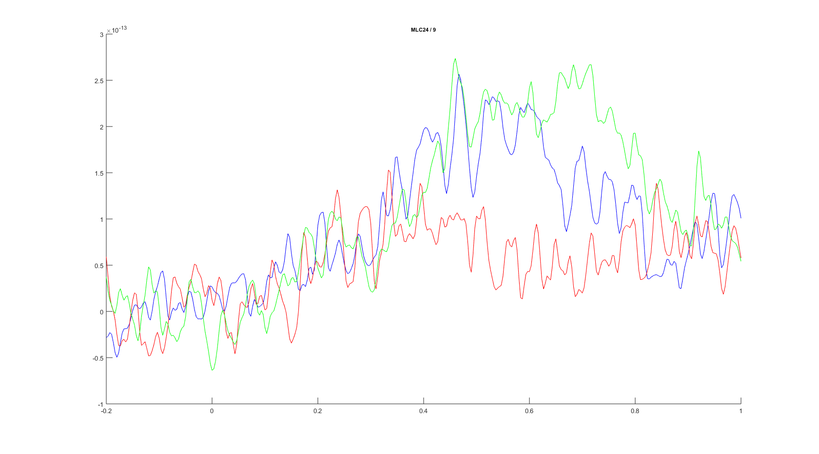
Figure 5; The event related fields plotted for three conditions for sensor MLC24 using ft_singleplotER

To plot the topographic distribution of the data averaged over the time interval from 0.3 to 0.5 seconds use to following commands:

cfg = [];
cfg.xlim = [0.3 0.5];
cfg.colorbar = 'yes';
ft_topoplotER(cfg,avgFIC)

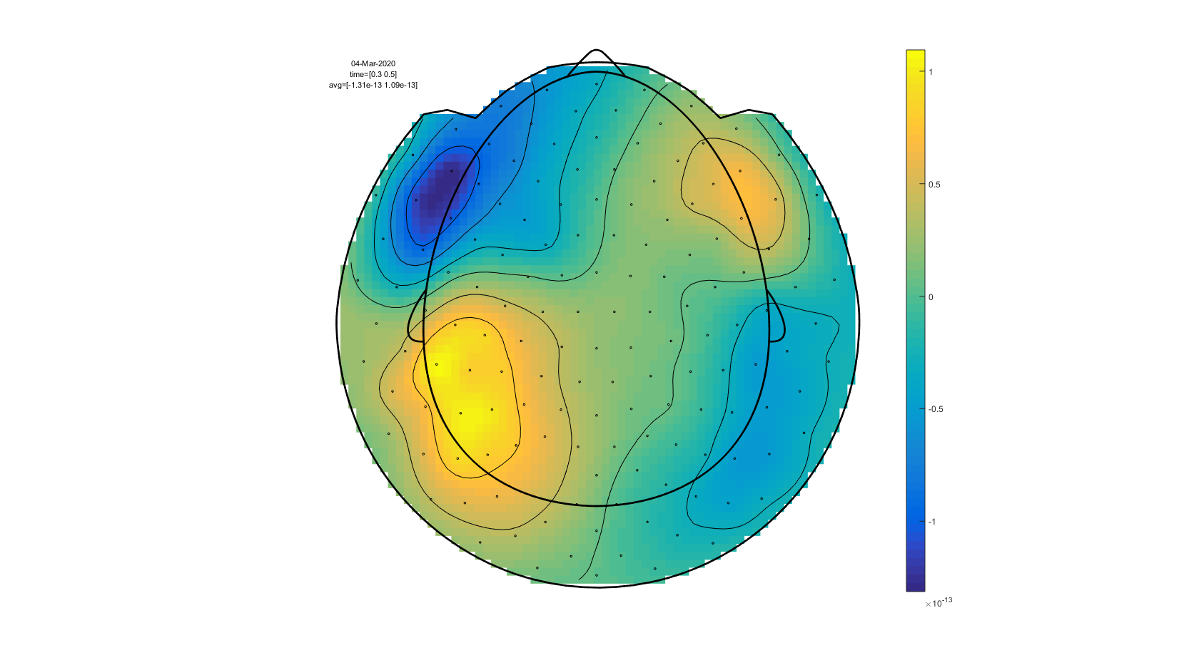
Figure 6; A topographic plot of the event related fields obtained using ft_topoplotER

To plot a sequence of topographic plots define the time intervals in cfg.xlim:

cfg = [];
cfg.xlim = [-0.2 : 0.1 : 1.0];  % Define 12 time intervals
cfg.zlim = [-2e-13 2e-13];      % Set the 'color' limits.
clf;
ft_topoplotER(cfg,avgFIC)

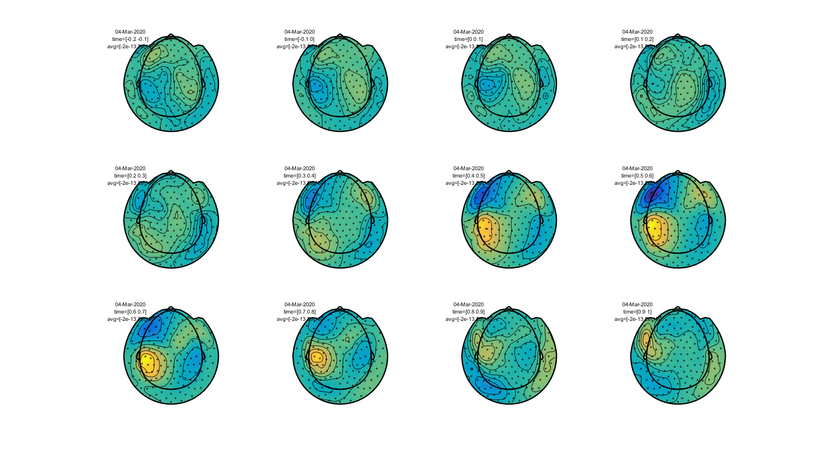
Figure 7; The topography of event related fields over time obtained using ft_topoplotER

Exercise 1 * What changes in data if you extend the baseline correction from -200 ms to 0 ms to -500 ms to 0?

• Apply a band-pass filter in the preprocessing instead of only a low-pass filter. Use for example the values from 1 to 30 Hz. What changes in the data? What are the pros and cons of using a high-pass filter?

Exercise 2

• Which type of source configuration can explain the topography?

With ft_megplanar we calculate the planar gradient of the averaged data. Ft_megplanar is used to compute the amplitude of the planar gradient by combining the horizontal and vertical components of the planar gradient;

The planar gradient at a given sensor location can be approximated by comparing the field at that sensor with its neighbors (i.e. finite difference estimate of the derivative). The planar gradient at one location is computed in both the horizontal and the vertical direction with the FieldTrip function ft_megplanar. These two orthogonal gradients on a single sensor location can be combined using Pythagoras rule with the Fieldtrip function ft_combineplanar.

Calculate the planar gradient of the averaged data:

cfg = [];
cfg.planarmethod = 'sincos';
avgFICplanar = ft_megplanar(cfg, avgFIC);

Compute the amplitude of the planar gradient by combining the horizontal and vertical components of the planar gradient according to Pythagoras rule:

cfg = [];
avgFICplanar     = ft_timelockanalysis(cfg, avgFICplanar);
avgFICplanarComb = ft_combineplanar(cfg,avgFICplanar);

To compare the axial gradient data to the planar gradient data we plot them both in one figure here

Plot the results of the field of the axial gradiometers and the planar gradient to compare them:

cfg = [];
clf
subplot(121)
cfg.xlim = [0.3 0.5];
cfg.zlim = 'maxmin';
cfg.colorbar = 'yes';
topoplotER(cfg,avgFIC)
colorbar
subplot(122)
cfg.zlim = 'maxabs';
ft_topoplotER(cfg,avgFICplanarComb)

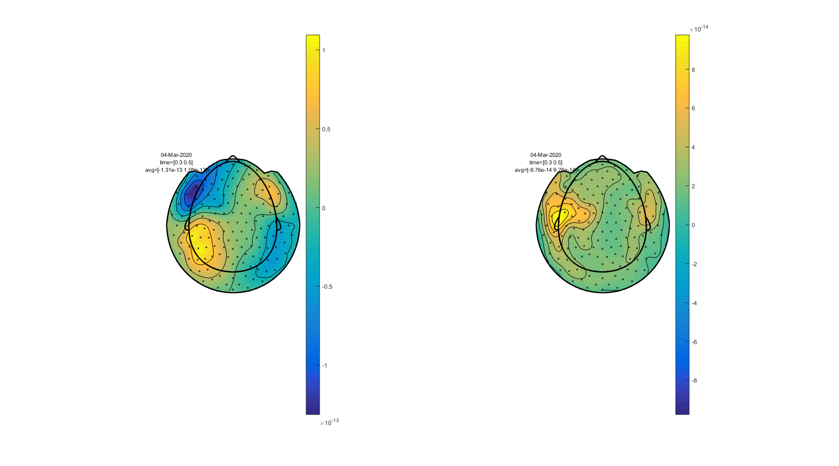
Figure 8; A comparison of event related fields from the axial gradiometers (left) and the planar gradient (right). The planar gradient was calculated using FT_MEGPLANAR and FT_COMBINEPLANAR.

Exercise 3

Compare the axial and planar gradient fields:

• Why are there only positive values above the sources in the representation of the combined planar gradient?
• Explain the topography of the planar gradient from the fields of the axial gradient

Finally you can make a grand average over all our four subjects with ft_timelockgrandaverage. Before calculating the grand average the data of each subject can be realigned to standard sensor positions with ft_megrealign.

For more information about this type the following commands in the matlab command window.

help ft_timelockgrandaverage
help ft_megrealign

This tutorial last tested with version 20100329 of FieldTrip.