FieldTrip

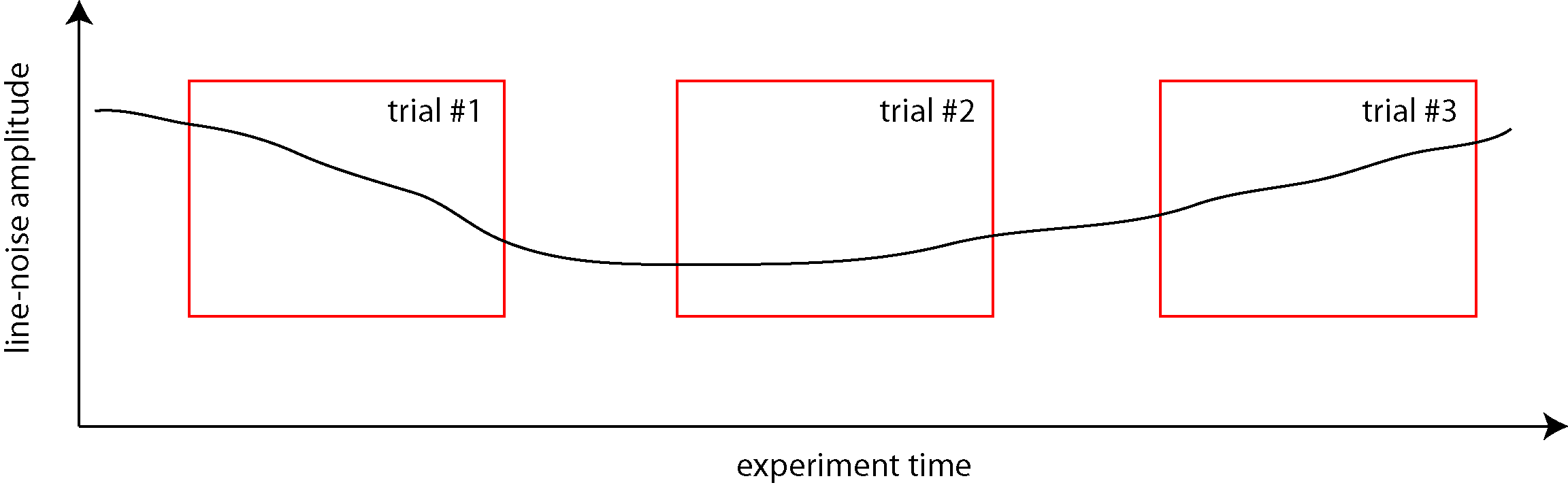
It is due to the non-stationarity of the line noise component in the data. Imagine a trial in which the 50Hz line noise increases in amplitude over time (e.g. trial #3 in the first figure).

If you fit a constant sine wave, its amplitude will be the mean, i.e. at the begin of the trial it will be larger than the actual amplitude and towards the end it will be smaller (second figure, using a 5 Hz example sine).

% time
t = (1:10000)/1000;
% frequency (Hz)
f = 5;         
% increasing amplitude
amp = (1:10000)/1000;

% 5 Hz sine with increasing amplitude
s1 = amp.*sin(2*pi*f*t);
plot(t, s1, 'b');

% dftfilter/ notch filter: fit 5 Hz sine (with constant amplitude)
avgamp = mean(amp);
s2 = avgamp.*sin(2*pi*f*t);
hold on; plot(t, s2, 'r');

Then imagine subtracting the estimated 50Hz component. At the begin you subtract too much, causing a negative (sign-flipped) 50Hz signal remaining in the data, and towards the end of the trial you are not subtracting enough, causing a positive (non sign-flipped) 50Hz signal remaining (black line in third figure). Over the whole interval, the 50Hz power is now zero. However, looking at a short piece at the begin, there is non-zero power at 50Hz. In the middle the power is small, but towards the end of the trial the power is again non-zero. I.e. the time-varying power is V or U shaped: large at the edges, small in the middle.

% subtract the 5 Hz fit
s3 = s1-s2;
figure; plot(t, s3, 'k'); 

% bandpassfilter: remove 4.9 to 5.1 Hz 
s4 = ft_preproc_bandpassfilter(s1, 10000, [4.9 5.1], 2);
hold on; plot(t, s4, 'm');  

After spectral estimation this would lead to a consistent decrease in 50 Hz towards the middle of the trials. Note that it depends on the spectral estimation technique and the data padding during filtering whether and how the residual line noise will express itself. An alternative approach would be to use a bandpass filter instead of the dftfilter (for result see magenta line in third figure).