Determine the filter characteristics
The following script demonstrates how you can determine the filter characteristics. Better ways than those described here are available, but this will give you an idea on how to approach the filter details. This snippet of code generates a one second piece of data with a delta function in it (i.e. a spike). This signal is passed though the ft_preproc_lowpassfilter function (located in fieldtrip/preproc) and the result is plotted in the time domain (left panel) and frequency domain (right panel).
% generate the signal and the corresponding time axis
s = zeros(1,1000); s(500) = 1; s = s - mean(s);
t = 0.001:0.001:1;

str = 'compare different cutoff frequencies';
clear f
f(1,:) = s;
f(2,:) = ft_preproc_lowpassfilter(s, 1000, 200);
f(3,:) = ft_preproc_lowpassfilter(s, 1000, 100);
f(4,:) = ft_preproc_lowpassfilter(s, 1000, 50);

figure;
subplot(1,2,1);
plot(t, f-repmat((0:3)',1,1000)); grid on; set(gca, 'ylim', [-3.5 0.5]); xlabel('time (s)'); ylabel(str);
subplot(1,2,2);
semilogy(abs(fft(f, [], 2).^2)'); grid on; set(gca, 'xlim', [0 500]); xlabel('freq (Hz)'); ylabel(str);

print -dpng fig1.png

  str = 'compare different filter orders (Butterworth)';
clear f
f(1,:) = s;
f(2,:) = ft_preproc_lowpassfilter(s, 1000, 50, 2);
f(3,:) = ft_preproc_lowpassfilter(s, 1000, 50, 8);
f(4,:) = ft_preproc_lowpassfilter(s, 1000, 50, 16);

figure;
subplot(1,2,1);
plot(t, f-repmat((0:3)',1,1000)); grid on; set(gca, 'ylim', [-3.5 0.5]); xlabel('time (s)'); ylabel(str);
subplot(1,2,2);
semilogy(abs(fft(f, [], 2).^2)'); grid on; set(gca, 'xlim', [0 500]); xlabel('freq (Hz)'); ylabel(str);

print -dpng fig2.png

str = 'compare Butterworth and FIR';
clear f
f(1,:) = s;
f(2,:) = ft_preproc_lowpassfilter(s, 1000, 50, [], 'but');
f(3,:) = ft_preproc_lowpassfilter(s, 1000, 50, [], 'fir');
f(4,:) = nan;

figure;
subplot(1,2,1);
plot(t, f-repmat((0:3)',1,1000)); grid on; set(gca, 'ylim', [-3.5 0.5]); xlabel('time (s)'); ylabel(str);
subplot(1,2,2);
semilogy(abs(fft(f, [], 2).^2)'); grid on; set(gca, 'xlim', [0 500]); xlabel('freq (Hz)'); ylabel(str);

print -dpng fig3.png

str = 'compare filter direction';
clear f
f(1,:) = s;
f(2,:) = ft_preproc_lowpassfilter(s, 1000, 50, [], 'but', 'onepass');
f(3,:) = ft_preproc_lowpassfilter(s, 1000, 50, [], 'but', 'onepass-reverse');
f(4,:) = ft_preproc_lowpassfilter(s, 1000, 50, [], 'but', 'twopass');

figure;
subplot(1,2,1);
plot(t, f-repmat((0:3)',1,1000)); grid on; set(gca, 'ylim', [-3.5 0.5]); xlabel('time (s)'); ylabel(str);
subplot(1,2,2);
semilogy(abs(fft(f, [], 2).^2)'); grid on; set(gca, 'xlim', [0 500]); xlabel('freq (Hz)'); ylabel(str);

print -dpng fig4.png
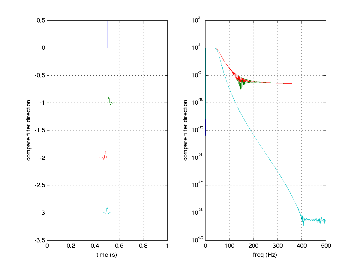
Note that the two-pass filter characteristic drops off twice as fast as the forward and reverse filter, even though the specified filter order is the same.