The correct pipeline order for combining planar MEG channels
Description
This script demonstrates the pipeline sequence you should follow when you use ft_combineplanar in your induced Time-Frequency and Event-Related Fields analysis. This script is specific for MEG datasets that have axial/magnetometer sensors (CTF, Elekta) and you’re interested to compute a synthetic planar representation.
Example dataset
It requires CTF275 gradiometer description data, which is available here
The following code creates a single dipole that projects brain activity on posterior sensors. We simulate an alpha component (10Hz) whose power decreases after a hypothetical visual stimulus delivery. The signal itself is not very important (you can design your own).
grad275 = ft_read_sens('ctf275.mat');

vol = [];
vol.r = 12;
vol.o = [0 0 4];

fsample = 500;
ntrial = 20;
smp = fsample*2; % 2 seconds epoch duration
time = -1:(1/fsample):1-(1/fsample);
f = 10; % signal frequency content

cfg=[];
for k=1:ntrial;
  amp = randn() + 1; % vary signal amplitude trial-by-trial
  endsig = randi([35,50],1); % vary randomly the begining of the alpha desynchronization
  t = linspace(endsig-100,endsig,smp);
  env = (-1./(1+exp(-t/(rand()+5)))) + amp; % inverted sigmoid function to simulate alpha desynchronization

  phi = randn()*0.5; % vary signal phase trial-by-trial
  signal = cos(f*time*2*pi + phi);
  cfg.dip.signal{k} = (env .* signal) + randn(1,smp); %power sigmoid envelope * oscillation + gaussian random noise
end

cfg.dip.pos   = [-1 -1 7]; %dipole located on posterior sensors
cfg.fsample   = fsample;
cfg.headmodel = vol;
cfg.grad      = grad275;
data_axial    = ft_dipolesimulation(cfg);
Time-Frequency analysis
Now let’s simulate how ft_combineplanar can or cannot influence the power output as a function of pipeline order. But first, it’s important to remind the logic behind the induced Time-Frequency Representation (TFR). What the induced TFR archives is the computation of the power estimates (non-linear transformation) for each single trial. As a consequence, the grand-mean (single-trials) of the induced TFR will add phase-locked PLUS non-phase-locked (time jittered) components. This is fundamentally different from the evoked TFR: first single-trials are averaged and then a TFR is computed. With the latter approach, non-phase-locked components wont be efficiently added because they’ll average out. More info in Tallon-Baudry et al 1996 J Neurosci
%% synthetic planar computation
cfg              = [];
cfg.feedback     = 'no';
cfg.method       = 'template';
cfg.planarmethod = 'sincos';
cfg.channel      = {'MEG'};
cfg.trials       = 'all';
cfg.neighbours   = ft_prepare_neighbours(cfg, data_axial);
data_planar      = ft_megplanar(cfg,data_axial);
With the ft_megplanar ‘sincos’ method, the vertical and horizontal components of each channel contain the negative and the positive parts of the signal. However, ft_combineplanar cfg.combinemethod = ‘sum’ for freq datatype, sums the power of the vertical and the horizontal components.
%% time-frequency analysis on axial and synthetic planar data
cfg            = [];
cfg.output     = 'pow';
cfg.channel    = 'MEG';
cfg.method     = 'mtmconvol';
cfg.taper      = 'hanning';
cfg.foi        = 2:1:40;
cfg.toi        = [0:0.05:2];
cfg.trials     = 'all';
cfg.t_ftimwin  = ones(length(cfg.foi),1).*0.5;
cfg.keeptrials = 'yes'; %% we keep the single trials
freq_planar    = ft_freqanalysis(cfg,data_planar);
freq_axial     = ft_freqanalysis(cfg,data_axial);

%% average the axial representation to compare later
freq_axial_avg = ft_freqdescriptives([],freq_axial);
Now let’s test the influence of pipeline order on the expected value
A) Combine planar for each single trial and then average
cfg               = [];
cfg.combinemethod = 'sum';
freq_combined     = ft_combineplanar(cfg,freq_planar);

freq_combined_avg1 = ft_freqdescriptives([],freq_combined);
The other way
B) Average single trials planar data (vertical and horizontal components) and then combine planar
freq_planar_avg = ft_freqdescriptives([],freq_planar);

cfg                = [];
cfg.combinemethod  = 'sum';
freq_combined_avg2 = ft_combineplanar(cfg,freq_planar_avg);
Let’s plot the results and see if there’s a difference
cfg         = [];
cfg.layout  = 'CTF275.lay';
cfg.channel = 'MEG';
cfg.xlim    = [0.5 1];
cfg.ylim    = [8 12];

figure;
subplot(321);ft_topoplotTFR(cfg, freq_axial_avg);title('axial');colorbar;
subplot(323);ft_topoplotTFR(cfg, freq_combined_avg1);title('combined-then-average');colorbar;
subplot(325);ft_topoplotTFR(cfg, freq_combined_avg2);title('average-then-combined');colorbar;

cfg         = [];
cfg.channel = {'MRO14', 'MRO24', 'MRO34', 'MRT27', 'MRT37'}; %right axial cluster
subplot(322);ft_singleplotTFR(cfg, freq_axial);title('axial');colorbar;

cfg.channel = {'MRO11', 'MRO12', 'MRO14', 'MRO22', 'MRO24', 'MRO31', 'MRO32', 'MRO34', 'MRT27', 'MRT37'}; %combined-planar cluster
subplot(324);ft_singleplotTFR(cfg, freq_combined_avg1);title('combined-then-average');colorbar;
subplot(326);ft_singleplotTFR(cfg, freq_combined_avg2);title('average-then-combined');colorbar;
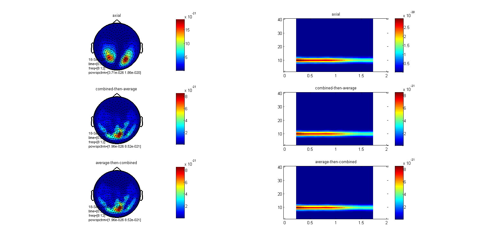
We can see that the second and the third row indicates that the other of the ft_combineplanar does not influence the power output (same topo and power scale). This is because with the induced TFR each single trial is squared (power estimate) and ft_combineplanar cfg.combinemethod=’sum’ on freq datatype sums the vertical and the horizontal components. As the single trial estimates are positive (power estimates), the order of the operation does not influence the output. You can now guess whether the same logic is going to hold for the Event-Related Fields.
Event-Related Fields
Now let’s going to play the same game but using Event-Related Fields (ERF). The logic underlying ERFs is to compute the mean over single trials (linear transformation) to disentangle the contributions of brain responses with fixed polarity and phase associated to specific events from random brain activity.
A) Combine planar for each single trial and then average
cfg               = [];
cfg.combinemethod = 'sum';
data_combined     = ft_combineplanar(cfg,data_planar); %% data_planar contains planar single trials

data_combined_avg1 = ft_timelockanalysis([],data_combined);
B) Average axial single trials, compute the planar gradient (vertical and horizontal components) and then combine i
data_axial_avg = ft_timelockanalysis([],data_axial); %% this is an Axial ERF

cfg              = [];
cfg.feedback     = 'no';
cfg.method       = 'template';
cfg.planarmethod = 'sincos';
cfg.channel      = {'MEG'};
cfg.trials       = 'all';
cfg.neighbours   = ft_prepare_neighbours(cfg, data_axial_avg);
data_planar_avg  = ft_megplanar(cfg,data_axial_avg);

cfg                = [];
cfg.combinemethod  = 'sum';
data_combined_avg2 = ft_combineplanar(cfg,data_planar_avg);
But as with the ‘sincos’ planar method the vertical and horizontal components preserve the positive and negative parts of the signal (it’s still not squared -> this is done in ft_combineplanar
C) Average planar (vertical and horizontal components) single trials and then combine
data_planar_avg = [];
data_planar_avg = ft_timelockanalysis([],data_planar);

cfg                = [];
cfg.combinemethod  = 'sum';
data_combined_avg3 = ft_combineplanar(cfg,data_planar_avg);
Let’s visualize and compare the result
cfg         = [];
cfg.layout  = 'CTF275.lay';
cfg.channel = 'MEG';
cfg.xlim    = [0.5 1];

figure;
subplot(421);ft_topoplotER(cfg, data_axial_avg);    title('axial');colorbar;
subplot(423);ft_topoplotER(cfg, data_combined_avg1);title('combined then average');colorbar;
subplot(425);ft_topoplotER(cfg, data_combined_avg2);title('average axial then planar+combined');colorbar;
subplot(427);ft_topoplotER(cfg, data_combined_avg3);title('average planar then combined');colorbar;

cfg = [];
cfg.channel = {'MRO14', 'MRO24', 'MRO34', 'MRT27', 'MRT37'}; %right axial cluster
subplot(422);ft_singleplotER(cfg, data_axial_avg);title('axial');

cfg.channel = {'MRO11', 'MRO12', 'MRO14', 'MRO22', 'MRO24', 'MRO31', 'MRO32', 'MRO34', 'MRT27', 'MRT37'}; %combined-planar cluster
subplot(424);ft_singleplotER(cfg, data_combined_avg1);title('combined then average');
subplot(426);ft_singleplotER(cfg, data_combined_avg2);title('average axial then planar+combined');
subplot(428);ft_singleplotER(cfg, data_combined_avg3);title('average planar then combined');
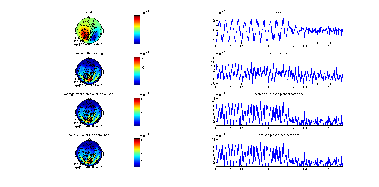
We can see that the second row (ft_combineplanar single trials and then average single trials) it’s very different (and way higher on amplitude) than the third and fourth rows. It’s very difficult to appreciate the alpha desynchronization effect (compare it with the axial representation, first row). This is because the ft_combineplanar cfg.combinemethod=’sum’ for raw and timelock data, squares the vertical and the horizontal planar components (non-linear transformation). Then, as ERF is a linear transformation (mean), the order of the non-linear transformation is going to influence the output. You can also see that if the average is computed on the axial and the planar level (both data representations preserve the positive and negatives parts of the signal), and then we combine the planar, the output is almost identical in time and space (topographies).